PAPER DEEP DIVE
Blind Precise Assembly: Proprioceptive Sim-to-Real Peg-in-Hole for Diverse Parts
Every robot already carries high-resolution contact sensors: its own joints. Legged robots and humanoids exploit them to walk, run, and track whole-body motions without vision, but there the contacts are large and forceful. Is joint sensing also enough for precise, contact-rich assembly, where the robot must find a millimeter-scale opening, mesh gear teeth, or catch a thread through light contact? We study this question by training blind assembly policies that observe only a short history of joint positions, velocities, and their own actions, without visual, force, torque, or tactile sensing. The poses of both the fixture and the part are unknown to the policy, and the grasp is randomized substantially. The policy must therefore assemble the parts through contact, sensed exclusively through its own proprioception. Trained with reinforcement learning entirely in simulation over randomized parts, grasps, and contacts, such policies learn peg insertion, gear meshing, and nut threading. The peg insertion policy transfers zero-shot to the real world and inserts pegs of different shapes and sizes in 73% of trials. Controlled comparisons with matched visual policies in simulation show that blind policies generalize far better to unseen part shapes and sizes, though they can be slower. Training such policies needs thousands of different assemblies, each simulated with its clearance intact, so we also release an open-source generator that builds them procedurally from exact convex pieces for MuJoCo; it is more accurate and faster than convex decomposition or MuJoCo's signed-distance collision. Videos and interactive simulations are at https://younghyopark.me/blind-proprioceptive-assembly/.
Paper: Blind Precise Assembly: Proprioceptive Sim-to-Real Peg-in-Hole for Diverse Parts
Authors: Antonia Bronars*, Younghyo Park* (*equal contribution), Kushal Kedia, Pulkit Agrawal — Massachusetts Institute of Technology
Link: https://arxiv.org/abs/2610.23849 (arXiv:2610.23849v1 [cs.RO], 16 October 2026, CC BY 4.0)
Project page: https://younghyopark.me/blind-proprioceptive-assembly/ (videos and interactive simulations)
Code status: released. mjfit, the procedural generator that builds MuJoCo assemblies from exact convex pieces, is at github.com/younghyopark/mjfit under the MIT licence and installs with pip install git+https://github.com/younghyopark/mjfit (Python 3.10+, MuJoCo 3.3+). The method-to-source correspondences below were read from commit eee986c, cloned on 19 October 2026. The policy-training code is not part of the release; training details come from the paper and Appendix A.
Real robot: Flexiv Rizon 4S (7-DOF) with a Robotiq 2F-85 parallel gripper, running at 50 Hz, with no real-world data and no fine-tuning.
In one sentence
Policies that observe nothing but 0.6 s of their own joint positions, joint velocities and previous actions — no camera, no force/torque sensor, no tactile skin, no fixture pose, no part model, no grasp estimate — learn peg insertion, gear meshing and nut threading from reinforcement learning entirely in simulation, and the peg policy transfers zero-shot to a real arm, seating 173 of 237 trials (73%) across eight printed pegs, three of them outside the training distribution. To make that training distribution possible the authors also release mjfit, which generates assemblies from exact convex prisms whose clearances survive contact: at 20 µm radial clearance it is an order of magnitude faster than MuJoCo's mesh SDF on CPU, while CoACD, V-HACD and mesh SDF all fill the clearance they are supposed to preserve.
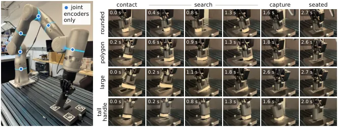
Figure 1 (paper Figure 1): blind insertion. A policy trained only in simulation inserts pegs of different shapes and sizes on a real robot using nothing but its joint encoders and its previous actions.
Background and motivation
A force applied anywhere on a robot's body travels through the links to the joints, which then move differently from what their commands alone would produce. The encoders record that difference, so the joints of every arm and leg double as contact sensors. Legged robots already exploit this: they walk, run and climb stairs blind, and humanoids use the same signal for whole-body motion tracking. In all of those settings, however, the contacts are large and forceful, and the joints often comply meaningfully while recording a measurable deviation.
Precise assembly sits at the opposite end of that spectrum. The robot must find an opening with a millimetre or less of clearance, bring gear teeth into mesh, or catch a thread — through light contact whose effect on the joints is easy to miss. The question this paper asks is whether the same proprioceptive channel carries enough information there. The authors answer it on three tasks: peg insertion, gear meshing and nut threading. On the real robot their insertion policy seats eight pegs of different cross-sections and sizes, three of them outside the training distribution, at 0.5–1.5 mm of clearance per side, in 73% of 237 trials — without being given the hole's location, the peg's pose in the grasp, the part's size, or its clearance. To the authors' knowledge this is the first such demonstration.
Prior insertion work takes one of three routes. Classical peg-in-hole combines compliance with search patterns — spirals, rasters, tilting — sometimes without force feedback at all, but these strategies assume a known grasp, a hole that lies within the pattern, and per-part tuning. Learned insertion policies usually add force/torque sensing, wrist vision, or both; a soft wrist with wrist force/torque sensing has reached 10 mm of hole-position tolerance and an unseen peg shape, and blind dexterous insertion has been shown with fingertip tactile sensing. A third group observes joint state together with a goal pose from perception or calibration, accurate to a few millimetres. This paper's policy is given none of those: no hole pose, no part model, no force signal, and an unknown pose of the part in its own grasp.
Training such robustness needs thousands of distinct assemblies, each simulated with its millimetre clearance intact — and that collides with a hard constraint of MuJoCo, which collides meshes through their convex hulls. A concave hole therefore needs either a signed-distance field or a set of convex pieces, and existing simulation benchmarks assemble those pieces from boxes by hand, which does not scale to random shapes. The automatic alternatives fail at these clearances: approximate convex decomposition (CoACD, V-HACD) tolerates concavity relative to mesh size, which is far larger than an assembly's clearance, so wall material ends up inside the hole; mesh SDF misses contacts and rounds the rim. The paper's Figure 5 makes this concrete — for the same parts, CoACD and V-HACD put material inside the hole and fill a nut's 0.1 mm thread clearance completely.
So the contribution is three things stacked: blind policies trained purely in simulation that learn all three tasks from proprioception alone, together with analyses showing that they search reactively rather than replay a fixed pattern and that they generalise to unseen part shapes and sizes far better than matched visual policies; the first sim-to-real policy for precise insertion from proprioception alone, transferring zero-shot and handling pegs outside its training distribution; and mjfit, an open-source procedural generator of MuJoCo assemblies with exact convex collision geometry, plus a benchmark against analytic ground truth in which it beats convex decomposition and MuJoCo's SDF collision on both accuracy and speed.
Preliminaries: observation, controller, simulator settings
Observation and action. The actor observes 33 values per step: seven joint positions, seven joint velocities, the gripper pose and twist computed from them by forward kinematics (twelve values), and its previous action (seven). The nut policy encodes gripper orientation with two columns of the rotation matrix instead of Euler angles, giving 36 values, because the wrist turns through half a revolution while threading and Euler angles would go singular. Actions are seven joint-position increments, scaled by the task's action scale and added to the measured joint positions, then tracked by a joint impedance controller $\tau=k_p(q_d-q)-k_d\dot{q}$. The peg task uses $k_p/k_d=80/20$ with a 0.02 rad action scale; gear and nut use $40/20$ with 0.04 rad (0.2 rad for the nut's wrist joint). Physics runs at 1 kHz under a 50 Hz policy, on an arm model whose armature, damping and friction were identified from real-world measurements — one of the reasons zero-shot transfer is plausible at all.
Temporal encoding. A temporal convolutional encoder compresses the last 30 observations (0.6 s) into a 32-dimensional latent $z_t$; an MLP with 256, 256, 128 units maps $z_t$ together with the current observation $o_t$ to joint targets. Everything the actor knows about the past must pass through that 32-dimensional bottleneck, which is precisely what makes the probing experiments in Section 3.2 meaningful: if the contact state were not in $z_t$, the policy could not be using it.
Simulator settings. Every benchmark scene uses a 1 ms step, the implicit-fast integrator, the Newton solver, $\mathrm{solref}=(2\,\mathrm{ms},1)$, $\mathrm{solimp}=(0.99,0.999,0.001)$, friction $\mu=1$ and zero margin. Baselines receive an exact watertight plate mesh (the circle tessellated at 1,024 segments, 0.04 µm sagitta) and ground truth is the analytic circle, so mjfit is charged for its own chord error and gets no accounting advantage. The peg is always an exact MuJoCo primitive, so every difference between methods comes from the hole side.
Method
1. mjfit: clearance as a first-class geometric object
mjfit automates the hand-built holes of simulation benchmarks and generalises them to arbitrary outlines. Given the planar outline of a hole, optionally with islands such as connector pins, it emits a ready-to-simulate MJCF model in which every contact surface is a MuJoCo primitive or a convex prism. The construction has three parts: the plate around the hole is split into convex polygons and extruded; the peg is the hole outline offset inward by the clearance, so every peg edge sits exactly one clearance from its hole edge; and islands become pockets in a hollow peg. Companion generators apply the same idea to bolt–nut pairs and spur gears, and a sampler draws random outlines, islands and dimensions, so a single training run can hold thousands of different assemblies.
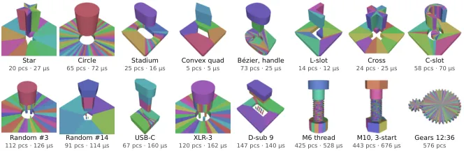
Figure 2 (paper Figure 4): assets generated by mjfit, one colour per convex piece of the collision geometry. Labels give the number of convex pieces (pcs) and CPU time per physics step with the parts in contact — a peg and its hole cost only a few dozen pieces.
The inward offset is mitred, not a naive vertex translation. In the source, offset_inward moves every edge of a counter-clockwise polygon inward along its normal by a distance $d$, mitring the corners, so the output has the same vertex count and topology and every output edge lies exactly $d$ from its input edge:
$$\mathbf{v}'_i=\mathbf{v}_i+d\,\mathbf{n}_{i-1}+t\,\mathbf{d}_{i-1},\qquad \begin{bmatrix}\mathbf{d}_{i-1} & -\mathbf{d}_{i}\end{bmatrix}\begin{bmatrix}t\\ s\end{bmatrix}=d\,(\mathbf{n}_{i}-\mathbf{n}_{i-1})$$
where $\mathbf{d}_i$ is the unit direction of edge $i$ and $\mathbf{n}_i$ its inward normal. When consecutive edges are collinear the matrix is degenerate and the code falls back to $\mathbf{v}_i+d\,\mathbf{n}_{i-1}$. The engineering value here is that "exact" is enforced rather than hoped for: an offset larger than the local feature size flips edges and folds the outline onto itself, and offset_is_valid detects both and raises, instead of silently producing a geometrically wrong peg.
# src/mjfit/_polygon.py — offset_inward (mitred)
for i in range(len(poly)):
    d_prev, d_curr = dirs[i - 1], dirs[i]
    a = np.column_stack([d_prev, -d_curr])
    b = distance * (inward[i] - inward[i - 1])
    if abs(np.linalg.det(a)) < TOL:
        out[i] = poly[i] + distance * inward[i - 1]    # collinear edges
    else:
        t, _ = np.linalg.solve(a, b)
        out[i] = poly[i] + distance * inward[i - 1] + t * d_prev
The peg–hole pairing in _peg.py is literally "the hole offset inward by the clearance", while islands are offset outward by the same clearance to become pockets, with checks at every step: each island must lie inside the hole, each pocket must fit inside the peg, and pockets must be pairwise disjoint (otherwise two islands are closer than twice the clearance). The wording of those errors is worth quoting, because it translates a manufacturing concept into a geometric one:
# src/mjfit/_peg.py — peg = hole offset inward; islands become pockets
hole_poly = source
insert = pg.offset_inward(hole_poly, c)
_check(pg.offset_is_valid(hole_poly, insert),
       f"clearance {clearance:g} m is too large for this hole: offsetting it inward "
       "by the clearance leaves no valid peg.")
for k, island in enumerate(isl):
    _check(pg.contains(hole_poly, island), f"Island {k} is not inside the hole.")
    pocket = pg.offset_outward(island, c)
    _check(pg.contains(insert, pocket), ...)
    for j, other in enumerate(pockets):
        _check(pg.disjoint(pocket, other),
               f"Islands {j} and {k} are closer than twice the clearance.")
The plate is cut into one convex wedge per hole edge. radial_wedges requires the hole to be star-shaped from its vertex mean, then builds a wedge per edge bounded by that edge, the two rays from the mean through its endpoints, and the plate boundary including any plate corners that fall between the rays. That yields far fewer pieces than a generic polygon triangulation, which is why a peg plus its hole stays in the "few dozen convex pieces" regime visible in Figure 2 — and piece count is exactly what determines per-step collision cost.
Curves are tessellated by circumscribed polygons, so the error direction is chosen deliberately. A circle of radius $R$ approximated by $n$ sides places its vertices at
$$r_n=\frac{R}{\cos(\pi/n)}$$
so the wall never intrudes into the true hole — the opposite of rings of boxes that inscribe the circle and therefore shrink it. The only error is extra play at the corners, which for an $n$-sided circle at radial clearance $c$ is
$$e_n=c\left(\frac{1}{\cos(\pi/n)}-1\right)$$
The side count is solved from a user-supplied error bound, $n=\max\!\left(6,\left\lceil \pi/\arccos\frac{R}{R+\varepsilon}\right\rceil\right)$. Combined with the fact that the construction knows which region must stay empty — so the user specifies the clearance directly instead of tuning a concavity tolerance and inspecting the result — this is the essential difference from approximate convex decomposition.
# src/mjfit/shapes.py — circumscribed polygon: side count and radius
def _sides(radius: float, max_error: float, minimum: int = 6) -> int:
    """Fewest sides whose circumscribed polygon stays within max_error."""
    if not max_error > 0:
        raise ValueError(f"max_error must be positive, got {max_error!r}.")
    half_angle = math.acos(radius / (radius + max_error))
    return max(minimum, math.ceil(math.pi / half_angle))

def circle(radius, *, n=None, max_error=MAX_ERROR, center=(0.0, 0.0), rotate=0.0):
    """Regular n-gon circumscribing a circle (first vertex on +x)."""
    n = _sides(radius, max_error) if n is None else int(n)
    a = np.linspace(0.0, 2 * np.pi, n, endpoint=False)
    r = radius / math.cos(math.pi / n)
    return _place(np.column_stack([r * np.cos(a), r * np.sin(a)]), center, rotate)
flowchart TD
  A["Planar outline of the hole
(optional islands: connector pins)"] --> B["Curves tessellated by
CIRCUMSCRIBED polygon
r = R / cos(pi/n)"]
  B --> C["Plate: radial_wedges
one convex wedge per hole edge
star-shaped from vertex mean"]
  B --> D["Peg: offset_inward by clearance c
mitred, same vertex count
every peg edge exactly c from its hole edge"]
  B --> E["Islands: offset_outward by c
become pockets in a hollow peg"]
  C --> F["Extrude to convex prisms"]
  D --> F
  E --> F
  F --> G{"offset_is_valid /
contains / disjoint checks"}
  G -->|fail| H["Raise: clearance too large,
islands closer than 2c"]
  G -->|pass| I["Ready-to-simulate MJCF
every contact face is a MuJoCo
primitive or convex prism"]
  I --> J["Sampler: random outlines,
islands, dimensions"]
  J --> K["12,288 parallel Warp worlds,
each holding a different assembly"]
Figure 3: generation pipeline drawn from Section 2.2 and the mjfit sources (_peg.py, _polygon.py, shapes.py). Two properties matter: the error only ever goes in the direction of extra play, and every geometric inconsistency raises at generation time instead of surfacing later as an unexplained jam in simulation.
2. The collision benchmark: passive probes with analytic answers
The paper does not stop at a qualitative claim of better geometry. It compares against the three automatic ways to give MuJoCo a concave hole — CoACD, V-HACD and MuJoCo's native mesh SDF — each swept over its own granularity setting, and plots speed against accuracy as Pareto fronts. The test bodies are 16 mm round and square holes in a 15 mm plate, with radial clearance $c$ from 200 µm down to 20 µm; at $c=20\,\mu\mathrm{m}$ the relative clearance is $2c/D=0.0025$. Threads use an M10 × 1.5 bolt and nut probed at 20 and 100 µm flank clearance. Errors are reported in micrometres of wall position, with negative values meaning phantom material stopped the peg early.
Five passive probes carry exact answers: a wall-offset probe (rays from the hole axis at 720 angles and 11 heights, no solver, ground truth the analytic outline), S0 contact onset (an aligned peg placed at known gaps, collision only, true onset at gap zero), S1 drop (a centred free peg dropped from 1 mm while $c$ sweeps from +1 mm to −500 µm, passing with zero wall contact if and only if $c>0$), S2 lateral play (planar slides, 0.1 N pushes in 24 directions, ground truth the support of the feasible translation set), S3 tilt play (slides plus one hinge at 1.5 mN·m, ground truth the maximum tilt at which both faces fit), and S4 yaw play (slides plus a vertical hinge for a square hole, ground truth $\arcsin\!\big(a/(s\sqrt{2})\big)-\pi/4$). One honest negative result is reported alongside them: at a 2 ms contact time constant, frictionless drops let pegs up to 20 µm oversize slip in for every method, exact geometry included, so S1 cannot resolve geometric errors below roughly 20 µm and the play probes must do that job. Stating the resolution limit of your own measurement is what makes a benchmark like this credible.
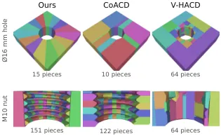
Figure 4 (paper Figure 5): the same parts under three decompositions, one colour per convex piece (Ø16 mm plate; M10 nut cut open). mjfit errs only toward extra play; CoACD and V-HACD put material inside the hole and fill the nut's 0.1 mm thread clearance.
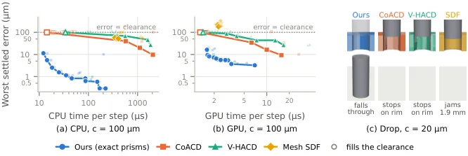
Figure 5 (paper Figure 6): speed against accuracy for a 16 mm round peg at 100 µm clearance, (a) on CPU with one environment on one thread and (b) on GPU, per-environment step across 256 MuJoCo Warp worlds with the error also measured on Warp. Each line is one method's Pareto front over all its settings; lower left is better and hollow markers fill the clearance (dotted line).
Paper Table 4 summarises the result — real-time factor at a 1 ms step with the peg pressed against the wall, ranges spanning each method's settings, GPU figures summed over 512 MuJoCo Warp worlds on one RTX 5090, and the last column giving the worst settled error at 20 µm radial clearance:
| Representation | CPU, 1 thread | GPU, 512 worlds | Error at $c=20\,\mu$m |
|---|---|---|---|
mjfit, square hole | 93× | 970× | 0.2 µm |
mjfit, circle, 7–32 sides | 82–29× | 1120–1070× | $\leq$ 2.6 µm |
mjfit, circle, 63–281 sides | 16–4.9× | 875–442× | $\leq$ 0.4 µm |
| Mesh SDF, octree depth 5–8 | 2.9–2.2× | 590–840× | fills, or 23–79 µm |
| CoACD, threshold 0.01 (839 hulls) | 1.8× | 254× | fills |
| Other CoACD and V-HACD settings | 3.3–70× | 680–1900× | fills |
Table 1: the collision benchmark (paper Table 4). Read it this way: on CPU mjfit is an order of magnitude faster than mesh SDF at equal or better accuracy (93× versus 2.9×), and on GPU it has the best speed–accuracy trade-off. Every convex-decomposition row says "fills" in the error column — at 20 µm those methods consume the clearance itself, after which their real-time factor is beside the point.
These errors change outcomes, not just numbers: a centred, aligned peg dropped from 1 mm stops on the rim or jams on every baseline's default plate, and falls cleanly through the mjfit plate (paper Figure 6c). And because each assembly is only a few dozen convex pieces, every one of the 12,288 parallel training worlds can hold a different one — the sentence that lets "diverse training distribution" and "exact clearance" hold at the same time.
3. Three tasks and what is randomised
All three tasks share a setup: a 7-DOF arm with a parallel-jaw gripper holds a part and must assemble it with a fixture that can sit almost anywhere in the workspace and can be tilted (paper Figure 3). Part geometry, pose in the grasp and contact properties are randomised and unobserved. Episodes start with the part already touching the fixture but misaligned, and succeed only when it is fully assembled, so the policy must both search for alignment through contact and then perform the assembly, from joint position feedback alone.
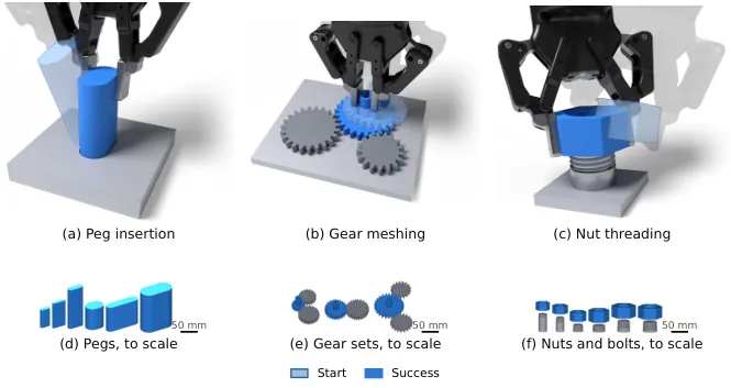
Figure 6 (paper Figure 2): peg insertion, gear meshing and nut threading. (a–c) The start of each task, faded, and the same grasp at success: the peg seated in its hole, the gear seated on its shaft in mesh with both anchor gears, the nut turned until its thread has caught. (d–f) Stadium pegs, gear sets and nuts and bolts generated by mjfit for training, to scale.
| Task | Part and clearance | Start state | Success / episode limit |
|---|---|---|---|
| Peg insertion | Stadium prisms with randomised cross-section, size, aspect ratio, mass and length; 1.0–1.5 mm clearance per side (0.5–1.5 mm for the deployed policy) | Peg touching the plate, a median 1 cm from the hole centre (2 cm for the deployed policy), tilted far more than the clearance admits | Entire peg bottom face seated / 5 s |
| Gear meshing | Involute spur gears, module 2.375–3.125 mm, 16–24 teeth; backlash 0.4–0.6 mm per anchor, bore clearance 0.75–1.0 mm | Gear resting on the shaft tip, off the shaft axis, teeth out of phase with the anchors | Bore surrounds the shaft and the gear sits within 1 mm of the collar, which meshing alone permits / 10 s |
| Nut threading | ISO metric nuts and bolts M24–M42, coarse and fine pitch; flank clearance 0.1–0.2 mm (0.05–0.2 mm full range) | Nut resting on the bolt tip, off axis and tilted, 87.5–142.5° of turning short of the thread catching | A quarter turn after the thread catches, nut within 1 mm of the bolt axis / 15 s |
Table 2: task definitions (Section 2.1 and Appendix A.1). The fixture centre is drawn within $x$ 0.54–0.76 m, $y$ −0.29–0.17 m, $z$ −0.20–0.29 m of the robot base with roll/pitch/yaw tilt of ±5° (±10° for the deployed policy); the grasp varies ±5.5 mm along the pads with ±10° in-hand tilt (±7 mm and ±20° deployed); plate friction 0.5–2.0, contact time constant 3.5–7.1 ms, finger friction scale 1.41–2.0 and gripper force cap scale 1.41–2.83 are all log-uniform. Geometry is drawn once per world, poses and contact parameters at every reset; no observation noise is added.
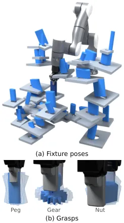
Figure 7 (paper Figure 3): training fixture poses and grasps. The gear and bolt fixtures span the peg's ranges, so all three tasks face the same order of positional uncertainty.
Rewards are sparse: a bonus on success plus one-time bonuses for intermediate milestones. For the peg these are the first capture by the opening and success (+1 each); for the gear, first capture of the shaft, first mesh with every anchor, and success; for the nut, seating, capture, each new extent of the turn, and success. Episodes also end early when the part moves far from the fixture, and nut episodes when the nut leaves the grasp.
4. PPO recipe and the asymmetric critic
Training uses PPO with every hyper-parameter stated: 12,288 worlds, 32-step rollouts, 5 epochs over 20 minibatches (24 for gear and nut), fixed learning rate $3\times10^{-4}$, clip $\varepsilon=0.2$, $\gamma=0.98$, $\lambda=0.95$, entropy coefficient 0.003, value-loss coefficient 1 with clipping, gradient norm clipped at 1, initial action standard deviation 0.5. The clipped surrogate and the advantage estimate are
$$L^{\mathrm{CLIP}}(\theta)=\mathbb{E}_t\Big[\min\big(r_t(\theta)\hat{A}_t,\ \mathrm{clip}(r_t(\theta),1-\varepsilon,1+\varepsilon)\hat{A}_t\big)\Big],\qquad \hat{A}_t=\sum_{l\geq 0}(\gamma\lambda)^{l}\delta_{t+l}$$
The first of two training-only accelerants is an asymmetric critic: it additionally sees the part's pose relative to the fixture, the true contact labels and, for the nut, the thread geometry, giving 240, 434 and 317 inputs for peg, gear and nut against the actor's 33 or 36. Privileged state reaches the critic only. The deployed peg policy adds two more things: a staged safety penalty, which starts once the task has been learned without safety limits and then penalises joint speeds and commanded torques above one sixth of the hardware limits, and an exploration anneal in which the learning rate adapts to a target KL of 0.01.
5. Contact supervision: privileged labels shape the latent, never the action
A blind policy has to infer contact from how the arm moves. To give that inference a dense training signal, the authors supervise the actor's latent with the contact state it cannot observe. At every step the simulator labels points sampled on the mating features of part and fixture as free, touching but misaligned, or aligned. For the peg, 64 points on the bottom edge are marked free (more than 1 mm above the plate's top face), in contact (on the rim or top face, within 1 mm), or inside the opening. For the gear, 64 points on the shaft's rim (free, on the gear, inside the bore) and 64 on the gear's tooth tips (free, on an anchor, in mesh). For the nut, 64 points on the rim of the bore (free, on the bolt tip, around the bolt, or caught by the thread within a band of 0.29 pitch — 1 mm at M30 × 3.5).
A small contact decoder with two hidden layers of 128 units predicts those labels from $z_t$, and its class-weighted cross-entropy is added to the PPO loss:
$$\mathcal{L}_{\mathrm{contact}}=-\frac{1}{64}\sum_{p=1}^{64}\sum_{k} w_k\,\mathbf{1}\!\left[c_{t,p}=k\right]\log \hat{p}_{t,p,k},\qquad (w_{\mathrm{free}},w_{\mathrm{contact}},w_{\mathrm{inside}})=(0.25,\,3.0,\,2.0)$$
The weights encode the class imbalance explicitly: almost every sampled point is free almost all of the time, while the few points in contact or caught are the ones that should determine the action, so free is down-weighted to 0.25 and contact raised to 3.0. The gradient of this loss trains the encoder only, and the prediction $\hat{c}_t$ never enters the policy — nothing privileged reaches the actor, and the decoder is simply dropped at deployment.
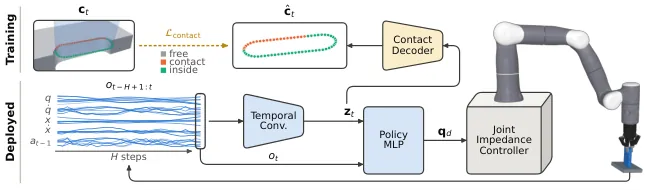
Figure 8 (paper Figure 7): policy architecture. A temporal convolution compresses the last $H=30$ proprioceptive observations $o_t$ (joint positions $q$ and velocities $\dot{q}$, gripper pose $x$ and twist $\dot{x}$, previous action $a_{t-1}$) into a latent $z_t$, and an MLP maps $z_t$ and $o_t$ to joint targets $q_d$ for a joint impedance controller. During training a contact decoder (amber) predicts the contact state $\hat{c}_t$ from $z_t$; its cross-entropy with the simulator's labels $c_t$ trains the encoder, but $\hat{c}_t$ never reaches the policy.
flowchart LR
  subgraph TRAIN["Training only (dropped at deployment)"]
    P["Privileged simulator state
part pose relative to fixture
64-point contact labels c_t"]
    DEC["Contact decoder
2 x 128 units"]
    LOSS["Class-weighted cross-entropy
w = 0.25 / 3.0 / 2.0
gradient trains the ENCODER only"]
    CRIT["Asymmetric critic
inputs: 240 peg / 434 gear / 317 nut"]
  end
  O["Observation o_t (33 values)
q, q_dot, gripper pose x and twist,
previous action a_t-1"] --> ENC["Temporal convolution
last H = 30 steps (0.6 s)"]
  ENC --> Z["Latent z_t (32-dim)
the only path from past to actor"]
  Z --> MLP["MLP 256 - 256 - 128"]
  O --> MLP
  MLP --> ACT["7 joint-position increments
scaled by action scale"]
  ACT --> IMP["Joint impedance controller
tau = kp (q_d - q) - kd q_dot
physics 1 kHz, policy 50 Hz"]
  IMP --> ROBOT["Arm model with identified
armature, damping, friction"]
  Z --> DEC
  P --> DEC
  DEC --> LOSS
  P --> CRIT
  ROBOT --> P
  ACT -->|"50 Hz, encoders only
no camera / F-T / tactile"| DEPLOY["Flexiv Rizon 4S + Robotiq 2F-85
frozen policy, zero-shot"]
Figure 9: the training-to-deployment dataflow, drawn from Section 2.3, Appendix A.1 and paper Figure 7. The point is that both privileged channels — the asymmetric critic and the contact decoder — exist only during training; at deployment the actor's input is still 33 encoder-derived values.
The second accelerant is measurable (paper Figure 14): without the contact loss the blind policies still learn all three tasks, but need 2.7× (peg), 3.8× (gear) and 5.1× (nut) as many environment steps to reach 90% training success. The unsupervised peg policy reaches 97.8% after 486M steps; the supervised ones pass 99% by 242M.
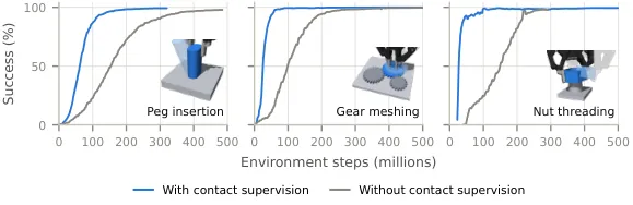
Figure 10 (paper Figure 14): contact supervision speeds up learning. Blue curves are the blind study policies with the contact loss, grey the same policies trained without it — the finer the task, the larger the benefit, with nut threading at 5.1× the steps.
6. Matched visual policies and the representation analyses
To isolate the sensing modality, the visual policies share the task, resets, randomisation, reward, actions and success check with the blind ones; the only difference is the input. A camera rigidly mounted on the wrist renders 64 × 64 RGB images of the held part and the fixture, the visual policy sees images only over the same 0.6 s history through a compact CNN, and both variants carry a 30-step history. The comparison is therefore not "memory versus no memory" but "memory filled by joints versus memory filled by pixels".
Two tools analyse what that memory holds. A linear probe: policies are rolled out in simulation, every state is labelled with one of seven task modes computed from the privileged part pose, and a linear probe $\hat{m}_t=\operatorname*{arg\,max}_k\left(W^\top z_t+b\right)_k$ is fitted to predict the mode from $z_t$. For the peg the modes are lifted, beside the plate, searching far, searching near (split at 5 mm from the opening), partly engaged, and fully inside either moving or stuck (inside but advancing less than 0.5 mm in 0.2 s); gear and nut modes follow their own task stages. Probes are trained on even-numbered worlds and tested on odd ones — 1.15M states from 1,536 worlds for the deployed peg policy, 133k and 85k states for the full-range gear and nut policies. A latent-swap test: a state keeps its own current observation but receives the $z_t$ of a state in another mode, and the action change is measured relative to a swap within the receiving state's own mode. Probing shows the latent contains mode information; swapping shows the policy actually acts on it.
Results
1. Proprioception is sufficient, and it costs time
All three tasks reach near-perfect success on in-distribution geometry: the blind peg policy 99.4% against 97.2% for the visual one, and blind gear and nut policies above 99.9% and at 99.7% respectively (the "In dist." column of paper Table 7). Joint history alone therefore carries enough information to find an opening, bring teeth into mesh and engage a thread.
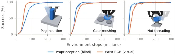
Figure 11 (paper Figure 8): proprioception alone is enough to learn all three tasks. Blind policies, which sense only their own joints, reach the same near-perfect training success as visual policies with a wrist camera. Lines are the mean of two training seeds.
The cost is time. On peg insertion the blind policy must find the opening through contact, so it follows a less direct path and seats later (paper Figure 9a, b). Appendix C's Table 5 prices that gap precisely:
| In-distribution behaviour (peg insertion) | Blind proprioceptive (ours) | Visual (wrist RGB) |
|---|---|---|
| Success (%) | 99.4 | 97.2 |
| Time to seat (s, median) | 0.80 | 0.44 |
| Insertions per minute | 65 | 82 |
| Lateral travel before seating (mm) | 37 | 20 |
| Time partly engaged (s) | 0.38 | 0.22 |
| Tilt when partly engaged / seated (°) | 6.7 / 1.1 | 5.2 / 1.1 |
Table 3: in-distribution behaviour (paper Table 5). Success, time and rate come from 8,192 episodes per seed averaged over both seeds; travel, engagement and tilt from the 3,964 of 4,096 matched starts where both seed-1 policies succeed. Medians unless stated; insertions per minute count every attempt, with failures charged their full 5 s. Starts lie a median 10 mm from the hole centre. The blind policy travels farther than the visual one from 99% of matched starts.
On the other two tasks the gap narrows and on gears it inverts: the blind gear policy seats in a median 0.58 s against the visual policy's 0.64 s, and is slower on only 43% of the 8,059 starts from which both succeed; the blind nut policy takes 0.76 s against 0.64 s and is slower on 98% of the 8,139 shared starts, by a median of 0.10 s. The authors' explanation is physical — the held part occludes the mating part from the wrist camera, so the visual policy has to search too. How much blindness costs therefore depends on how badly the grasp occludes the fixture.
2. Visually blind but intelligent
The probes agree across tasks. Balanced accuracy over the seven modes (chance 14%) is 70% for the peg — against 56% from the current observation alone and 33% from a randomly initialised encoder — 61% for the gear (41% / 29%) and 73% for the nut (64% / 46%). The history latent beats the instantaneous observation everywhere, so the information lives in the 0.6 s window rather than in a single frame. For the peg, the history latent recognises lifted, moving and stuck states with 84–90% recall; its characteristic mistakes are decoding far search as near 19% of the time and near as far 26% — two modes that call for nearly the same action, so the confusion is cheap.
| Task | From history latent $z_t$ | From current observation $o_t$ | From random encoder | Chance |
|---|---|---|---|---|
| Peg insertion (deployed policy, 1.15M states) | 70% | 56% | 33% | 14% |
| Gear meshing (full-range policy, 133k states) | 61% | 41% | 29% | 14% |
| Nut threading (full-range policy, 85k states) | 73% | 64% | 46% | 14% |
Table 4: linear-probe balanced accuracy (Appendix C, "Probe details"). Probes are fitted in simulation only, trained on even-numbered worlds and tested on odd ones.
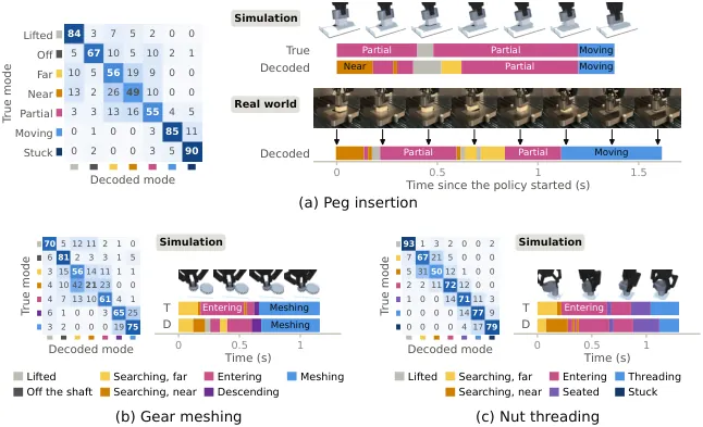
Figure 12 (paper Figure 10): the blind policies' joint histories encode the task's mode, in simulation and on the robot. A linear probe fitted only in simulation reads the mode from each policy's history latent; each matrix gives its confusions (%), and beside it one start state is decoded at every step (T: true mode, D: decoded). On all three tasks the probe cleanly separates modes that call for different actions, such as lifted, engaged and stuck. (a) On the robot it decodes the same sequence of peg-insertion modes as in simulation.
The latent-swap test supplies the causal half: swapping the latents of a searching state and an inside state changes the action 1.4–1.9× as much as a swap within the same mode, while swapping near against far search changes it only 0.99–1.11×. For the gear the corresponding figures are 1.3–1.6× (searching against engaged) versus 0.97–1.04× (near against far); for the nut, 1.4–3.0× versus 0.94–1.18×. The latent therefore encodes precisely those distinctions that require a different action — which is what separates reactive search from a replayed script.
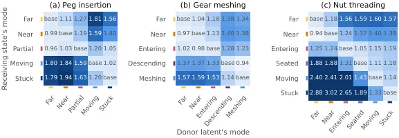
Figure 13 (paper Figure 15): the latent-swap test. Each state keeps its own current observation but receives the history latent $z_t$ of a state in another mode; every cell is the mean change in action relative to a swap within the receiving state's own mode. Cross-mode blocks are visibly hotter while near-against-far sits around 1.
Reacting to contact also makes blind assembly cheaper in path length. A fixed pattern sweeps the same route regardless of what the arm feels, whereas a reactive policy can use what contact told it — for instance that the peg caught the rim — to steer the search. The paper tests this against the standard scripted blind baseline for insertion under position uncertainty, spiral search: from the same starts the blind policy travels a median 37 mm before seating, against 95 mm for an optimistic spiral that starts flush with the hole opening and is handed the peg's orientation and the best starting direction.
The probe also transfers to the robot, and in doing so exposes the sim-to-real seam. Running 30 further trials on peg I3, actions recomputed from the logged observations match the logged ones to within $2\times10^{-5}$, so the deployment pipeline itself introduces no drift. At the end of successful trials, however, the peg pose estimated from joint encoders and the planned grasp sits a median 6.6 mm (10th–90th percentile 2.6–17.4 mm) from the seated pose, because the peg slips and turns in the fingers, and it places only 3% of those states fully inside the hole. The probe labels 62% of inside states correctly against 100% in simulation from the same starts, and labels the final state of 17 of 24 successful trials as inside. For the start state shown in Figure 12a, true and decoded modes agree on 74% of steps in simulation (median 65% over the 30 start states).
3. Blind generalises to unseen parts far better than vision
This is the heaviest comparison in the paper. The protocol widens exactly one part property beyond the study training range while every other range stays at its study value: a tighter fit; mild and strong changes of proportions (aspect ratio, tooth height, thread depth); mild and extreme changes of size on both sides of the training range; and a new shape (random convex peg outlines, random quadrilateral gear teeth, random 5–8 sided nuts).
| Task / sensing | In dist. | Tighter | Proportions, mild | Proportions, strong | Size, mild | Size, extreme | Random shape |
|---|---|---|---|---|---|---|---|
| Peg insertion · proprioception (blind) | 99.4 | 93.8 | 97.1 | 93.3 | 97.1 | 91.9 | 36.2 |
| Peg insertion · RGB (visual) | 97.2 | 54.1 | 62.7 | 40.1 | 57.7 | 16.4 | 3.9 |
| Gear meshing · proprioception (blind) | >99.9 | >99.9 | >99.9 | >99.9 | >99.9 | >99.9 | >99.9 |
| Gear meshing · RGB (visual) | 98.4 | 98.0 | 98.6 | 98.5 | 96.5 | 90.2 | 87.9 |
| Nut threading · proprioception (blind) | 99.7 | 99.2 | 99.2 | 98.2 | 98.8 | 98.4 | 99.7 |
| Nut threading · RGB (visual) | 99.7 | 98.7 | 99.1 | 98.8 | 25.5 | 1.6 | 57.1 |
Table 5: success on unseen parts in % (paper Table 7), one column per bar of paper Figure 11. Peg insertion is the mean over two training seeds per policy, gear and nut one seed; both policies use a 30-step history. The starkest cells are the nut's size columns (visual 25.5% and 1.6% against blind 98.8% and 98.4%) and the peg's random-shape column (visual 3.9% against blind 36.2%).
The reading is direct: a visual policy learns to align visual features that may not appear in held-out assemblies, while a blind policy learns a search strategy that depends on the part only through its contacts and therefore transfers. Blind is not immune either — 36.2% against 99.4% is still a cliff on random convex pegs, whose median area is only 53% of the matching stadium's — but it is an order of magnitude above 3.9%. The full-range policies stay reliable on held-out instances of their own distribution: with deterministic actions the gear policy succeeds in 98% of 8,192 episodes over 4,096 unseen gear sets, and the nut policy in 93% of 8,192 episodes over 512 unseen nut-and-bolt pairs.
4. Zero-shot on the real robot: 173 of 237 trials
The frozen blind policy runs on a Flexiv Rizon 4S with a Robotiq 2F-85 at 50 Hz, with no real-world data and no fine-tuning, receiving only encoder-derived joint and gripper state — no camera, no force/torque sensor and no hole pose enters the policy. The deployed variant is the one trained on random convex, smooth and mixed cross-sections under a handle. Eight 3D-printed pegs are tested: five in-distribution objects and three drawn from outside it, with a tighter 0.5 mm per-side clearance, a larger cross-section, and a taller handle. Each trial starts from a state drawn from the simulated reset distribution, the peg grasped at a randomised position and tilt and touching the fixture near the hole, and an operator marks success once the peg is seated.
| Peg | Category | Geometry and clearance | Success |
|---|---|---|---|
| I1–I5 | In distribution | Cross-sections drawn from the deployed policy's training distribution (polygonal, smooth, mixed), 1.11–1.49 mm clearance per side, under an 80 × 44 mm stadium handle 40 mm tall | 73–80% each |
| C | Out of distribution: tighter | Polygonal peg with 0.5 mm clearance per side, below the study training range | 66% |
| L | Out of distribution: larger | A training outline enlarged by 1.28 × 1.09 to a 101 × 37 mm hole | 66% |
| H | Out of distribution: taller handle | Mixed outline under a 70 mm handle (40 mm for the others) | 72% |
| Total | Pegs weigh 147–164 g and every hole is 20 mm deep; 30 planned resets per peg, each reset counted once by its first attempt that reached a verdict — operator success or failure, or the 20 s horizon, which counts as failure | 173 / 237 = 73% | |
Table 6: real-world results (Section 3.4, paper Figure 12, Appendix C "Real-world pegs"). Each simulated rate is the same policy over 2,048 worlds of that peg's geometry at the same 20 s horizon with deterministic actions; error bars are 95% Wilson intervals. On the robot the policy presses onto the surface, sweeps, and drops in once the opening is under the peg — the same behaviour as in simulation.
What stands out is how small the gap is between the three out-of-distribution pegs (66%, 66%, 72%) and the five in-distribution ones (73–80%), given that the policy has no hole pose, no part model and a randomised grasp. Compared with the visual collapse in Table 5, this is the transfer-side confirmation of the same claim.
Limitations
Stated by the authors: it is a last-mile skill that assumes it starts in contact. Every training episode begins with the peg already touching the fixture a few centimetres from the hole, so some other motion, scripted or visual, must bring it there. That bounds the claim: the method solves "find the hole and seat the peg once you are already on the plate", not "pick a peg from a bin and register it".
Stated by the authors: the behaviour is local. The policy searches the surface around where it starts and corrects the misalignments it met in training, but it cannot handle events that call for more than a local correction, such as a peg that slides out of the grasp and lands far from the hole.
Added here: how the real-world verdicts were produced, and how narrow they are. Real-robot success is judged by an operator under a 20 s horizon, and the physical demonstration covers peg insertion only — gear meshing and nut threading are never transferred, so the striking generalisation gap in Table 5 is measured entirely in simulation. With 30 planned resets per peg, the difference between 66% and 73% is not large enough to support a strong claim that out-of-distribution pegs are as easy as in-distribution ones.
Added here: throughput is traded away without a fusion baseline. 65 against 82 insertions per minute and 0.80 against 0.44 s to seat are not neutral on a production takt time. The paper buys robustness to unseen geometry with that time, but it never evaluates the hybrid that engineering would most likely ship — vision for coarse approach, proprioception for the last millimetre.
Added here: on the robot the probe reads contact indirectly. Inside-state recall drops to 62% against 100% in simulation, the estimated end pose sits a median 6.6 mm from the seated pose, and only 3% of those states are judged fully inside. Real-robot mode decoding therefore leans on an estimate of grasp slip, making the robot-side probe evidence correlational; the causal latent-swap experiment was run in simulation only.
Added here: mjfit's error direction and its speed price. Circumscribed tessellation errs only toward extra play, which is safe for training but means the effective clearance slightly exceeds the nominal one at the 20 µm scale (controlled by $e_n$ through the side count). Accuracy and speed also remain a user-side trade-off: going from 7–32 sides to 63–281 sides on a round hole drops the CPU real-time factor from 82–29× to 16–4.9× while tightening the error from ≤2.6 µm to ≤0.4 µm.
Takeaways and what comes next
The contribution is not "yet another insertion policy" but the overturning of a default assumption: precise assembly does not require vision or force/torque sensing. Joint encoders under light contact, combined with wide randomisation and a 32-dimensional temporal bottleneck, suffice to search for a millimetre-scale opening, align gear phases and catch a thread. Just as useful is the methodology for showing this is not a rehearsed script — a linear probe to demonstrate that the latent carries the contact mode, and a latent swap to demonstrate that the policy acts on it. Those two together form an evidence chain that can be applied to any policy claimed to have learned a contact skill.
For teams working in simulation, mjfit is usable today: pip install git+https://github.com/younghyopark/mjfit, with a CLI offering mjfit peg --shape star, mjfit peg --config usb_c (a bundled USB-C receptacle with its tongue), mjfit thread --config m10 and mjfit gear --teeth 18 24, while the Python generators return MJCF strings. The problem it solves is specific and familiar: when you need thousands of assemblies with exact clearances, convex decomposition eats the clearance and mesh SDF misses contacts at an order-of-magnitude speed penalty. Its treatment of clearance — let the user name it, define the peg as the hole offset inward, tessellate curves by circumscription — is a reusable design principle: in precise-assembly simulation the direction of a geometric error matters more than its size, and a method that errs only toward extra play is safe to train on.
The natural next steps follow the boundaries the authors draw: attach an approach policy, visual or scripted, to the last-mile skill so the pipeline starts from a bin rather than from contact; port the contact-supervision recipe — an auxiliary loss that accelerates sparse-reward learning without giving the actor privileged information — to other contact-rich tasks such as connector insertion, snap fits and wire routing; use the probe as a deployment-time contact-state monitor, since it already decodes the same mode sequence on the robot while its 62% inside recall marks exactly where sim-to-real still leaks; and push the gear and nut policies onto hardware to see how much of that above-99.9% and 98% simulated generalisation survives real threads.
Golden quote
"Every robot already carries high-resolution contact sensors: its own joints."
The opening line of the abstract. Legged robots and humanoids already exploit that channel to walk, run and track whole-body motion without vision — but there the contacts are large and forceful. This paper asks whether the same channel survives the regime of light contact and millimetre clearance, and answers yes.