HuMBLE: Human Motion-Driven Behavior Learning for Embodied Locomotion

HuMBLE: Human Motion-Driven Behavior Learning for Embodied Locomotion
Mike Zhang, Dongho Kang, Kevin Bergamin, Nicola Burger, Robin Deits, Jonathan Foster, Bilal Hammoud, Katie Hughes, Francesco Iacobelli, Twan Koolen, M. Eva Mungai, Zach Nobles, Shane Rozen-Levy, Jean Pierre Sleiman, Fangzhou Yu, Yunbo Zhang, Alfred Rizzi, Jessica Hodgins, Scott Kuindersma, Yeuhi Abe, Sylvain Bertrand, Farbod Farshidian (RAI Institute / Boston Dynamics / Carnegie Mellon University; corresponding author Dongho Kang, dkang@rai-inst.com)
arXiv:2610.10489v1 [cs.RO], submitted 2026-10-07 · arXiv:2610.10489 · License CC BY 4.0
Code status: the paper lists no public code repository and no project page. The authors state that the human motion dataset collected for this work (roughly three hours of motion capture, including a 0.8x pre-scaled variant aimed at smaller humanoids) will be released, but the main text gives no release date. Of the three validation platforms, the joint-level PD gains for Boston Dynamics Atlas R1 / D1 are withheld under proprietary agreements; the full Unitree G1 parameter set appears in supplementary Table S7.

The Takeaway in One Sentence

HuMBLE splits "looks human" from "obeys commands" into two stages: a privileged teacher policy trained with RL against a full-body reference produces dynamically feasible motion, which is then distilled into a student prior that sees nothing but proprioception plus one SE(2) velocity command; that prior is fine-tuned by running short-horizon reference-imitation environments and long-horizon goal-commanded environments side by side, which pushes command coverage past the edge of the data distribution without surrendering style. The final policy is a single MLP(1024,1024,1024) that infers in 1.1 ms on the Jetson AGX Orin CPU of a Unitree G1, absorbs pushes up to 1400 N along the principal directions on Atlas R1, and degrades data fidelity relative to its teacher by only 20.83% (linear velocity) to 130.31% (angular velocity), where a single-stage command-conditioned policy degrades sidestepping by 240.87% and simply stops answering the steering command.

1. The Problem: Style and Command Coverage Pull Against Each Other

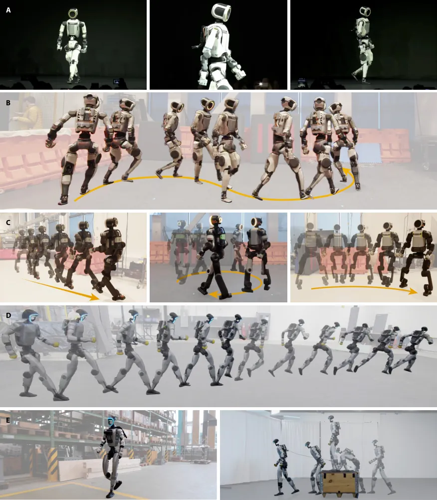
Figure 1 (paper Figure 1): hardware results across the three platforms. (A) Atlas R1 in a staged public demonstration; (B) Atlas R1 following a continuously varying real-time turning command; (C) Atlas D1 walking backward, circling, and sidestepping, showing coverage of the SE(2) command space; (D) Unitree G1 spontaneously switching from walking to sprinting as commanded speed rises; (E) HuMBLE used as the low-level locomotion module inside hierarchical stacks for autonomous navigation (left) and box parkour (right).

Humanoid walking is treated as a core benchmark not only because it is hard, but because it is behavior other people can read at a glance. The introduction makes that thread explicit: from ASIMO's cautious footsteps in the early 2000s to PETMAN's forceful gait in the 2010s, humanoid locomotion has carried social signaling duties. Step timing, body motion, and velocity transitions are cues that people interpret through their own priors from human-human interaction, so legibility, trust, and usability all improve when a robot walks like a person.

The difficulty is that "looks human", "driven by real-time commands", and "reliably deployable on hardware" are three requirements that existing routes usually satisfy only two at a time. The paper states the three conditions a deployable controller must meet simultaneously: preserve the stylistic quality of human locomotion and natural gait transitions across speeds and directions; respond accurately and stably to a broad range of user-specified velocity commands; and execute with low enough latency, memory, and compute to run onboard.

The first route is first-principles control and motion generation: heuristic motion generation, high-level motion features, biomechanically derived control objectives, and today's model predictive control and reward-engineered RL. These methods are genuinely strong at command tracking, balance, and disturbance recovery. But human gait depends on tightly coupled whole-body coordination, subtle differences in contact timing, arm and leg swing trajectories, posture, and gait transitions that change with speed and direction; encoding all of that in hand-designed objectives does not scale. The result is controllers that track and recover well while looking mechanical.

The second route uses human motion data directly as supervision. In character animation this runs from motion graphs and interactive motion synthesis through Motion Matching, and more recently toward VAEs, GANs, diffusion, and flow matching: motion data is treated as samples from a reference distribution, so the objective shifts from reproducing a trajectory to aligning a synthesized distribution with the reference one. VAEs in particular are widely used to embed high-dimensional motion into structured latent spaces for higher-level policies to explore, and the idea has been adapted to legged robots by coupling VAE-based generators with RL trackers or by conditioning policies on learned gait embeddings. The cost is that these methods struggle to reproduce the kinematic structure and contact consistency of the demonstrations, and artifacts such as foot slip and unnatural joint configurations directly undermine physical plausibility.

The third route is adversarial imitation learning. It skips the two-step "generate kinematic motion, then track it separately" pipeline and instead uses a discriminator reward to judge how close the executed behavior is to the demonstration, optimizing until the two are indistinguishable. AMP is the representative case: an RL policy consumes both a task reward for command tracking and a discriminator style reward derived from motion data, and it has produced stylized, steerable gaits on quadrupeds and humanoids. ASE and CALM add skill embeddings and hierarchical control to fight mode collapse and preserve behavioral diversity. The problems are also clear: min-max training is sensitive to reward scaling, discriminator design, and hyperparameters, and a learned style reward only influences behavior indirectly, which makes fine-grained user control over the emergent motion awkward.

Most recently, diffusion and flow matching have been pushed into physical control, mapping robot state and commands straight to actions and removing the separate tracking layer. Expressiveness is not the issue; iterative sampling or numerical integration is hard to reconcile with the latency, compute, and power budget of onboard real-time control.

Set these routes side by side and the paper's choice becomes clear: the training instability of adversarial and generative formulations, their indirect behavioral control, and their runtime inference overhead are all disqualifying for low-latency onboard humanoid control. HuMBLE therefore writes the problem as a partially observable Markov decision process (POMDP) in which the full-body reference state exists as privileged information during training but is unavailable to the deployed policy. At runtime the policy tracks no whole-body reference trajectory at all. Instead it learns to reconstruct coordinated whole-body behavior from proprioception and the user's SE(2) velocity command, and emits joint-level actions directly.

Teacher-student distillation alone leaves one problem standing: the policy is trained strictly inside the support of the reference data, so command coverage is bounded by that data. Issue a command at deployment that is missing or sparse in the dataset and you get an out-of-distribution failure. "Fast diagonal walking" combined with "high turning rate" is exactly such a case: a joystick reaches it effortlessly, human walking rarely does. The paper's answer borrows the pretrain-then-post-train pattern from foundation models, except the post-training is not plain goal-conditioned fine-tuning. It is a structured multi-task RL: short-horizon reference-guided imitation anchors the policy to the human motion manifold, long-horizon goal-conditioned command tracking pushes responsiveness and robustness beyond the data support, and a goal-conditioned state initialization scheme keeps the whole thing stable.

The central claim compresses to one sentence: separate style acquisition from command-space expansion. Style is held by an explicit reference-tracking reward rather than by some learned latent style objective, which makes the balance between the two directly interpretable. The environment allocation ratio in stage two is a knob you can turn.

2. Preliminaries: The Whole-Body Reference as Privileged Information

Four existing building blocks are needed to follow the pipeline. The first is the teacher-student architecture. In legged robotics it is usually deployed against partial observability, most often rough-terrain walking: terrain geometry is fully visible in simulation but only partially or not at all observable on hardware, so a teacher that can see the terrain learns first and is distilled into a student that cannot. The usage closest to this paper is in physically simulated characters, where diverse human-like behaviors conditioned on high-level user commands are learned from human motion data.

The second is the motion imitation framework introduced by ZEST. The teacher policy here is trained directly in that setting: comparable observation spaces, reward structure, termination conditions, and an auxiliary torque curriculum. Joint-level PD gains also follow the ZEST procedure, designed from each joint's projected motor armature value.

The third is reference state initialization (RSI): when an episode terminates, either by running through the reference clip or by early termination for deviating too far from it, a state is sampled from the reference data, perturbed around that sample, and used as the initial condition of the next episode. The fourth is DAgger: states come from the student's own rollouts, the teacher is queried for the action it would have taken at each of those states, and the answers become supervised labels, so the training distribution follows the student's state distribution rather than the teacher's.

3. The Dataset: 528,214 Frames With Per-Frame SE(2) Command Labels

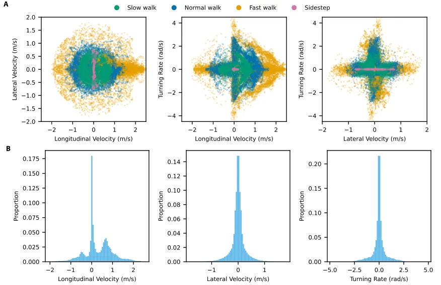
Figure 2 (paper Figure 7): distribution of the annotated commands in the dataset after retargeting to Atlas R1. Only the standard walking regime is plotted so the densest region stays readable; high-speed sprinting data exists separately. (A) Command scatter for four modes, fast forward walk, normal forward walk, slow forward walk, and sidestep, decimated by a factor of 10 for readability; (B) marginal histograms of longitudinal velocity, lateral velocity, and turning rate, with the vertical axis showing frame fraction relative to the dataset size N=528,214. The sparse "lateral velocity combined with turning rate" corner that Section 7 has to fix is the palest region of this plot.

Motion was captured with a Vicon optical system at 120 Hz, with the marker set and character skeleton calibrated to the actor's own body dimensions and range of motion. Raw marker trajectories were post-processed first: missing markers were filled by interpolation and skeleton kinematic constraints, then filtered to remove high-frequency noise; the character skeleton was fitted to the cleaned marker data and exported as BVH.

The choreography was designed around coverage of the SE(2) torso velocity space, in five speed regimes (slow walk, normal walk, fast walk, jog, sprint), reusing the same set of "dance cards" inside each regime so SE(2) trajectory coverage stays consistent across speeds. The structured scripts fall into four families: discrete turns through an eight-direction star (0, +/-45, +/-90, +/-135, 180 degrees); continuous tracking of spiral splines, used to sweep a continuum of curvature radii; straight-line maneuvers (starts, hard stops, direction reversals, lateral translation); and in-place turns at zero linear velocity that begin and end on the same eight headings. Beyond the structured takes there is unstructured data captured specifically for natural transitions between speeds, turns, stops, and starts. The method is to shout random verbal cues at the actor at random intervals (start, stop, turn, walk fast, walk slow), so a high-entropy instruction sequence suppresses the actor's own subconscious preferences. Data collection was also iterated against observed capability gaps during development, for example re-collecting a batch of sidestepping when sidestep performance lagged.

Getting from BVH to robot trajectories takes a two-stage retarget. Stage one maps the animation onto a kinematic proxy skeleton: human-style ball-joint topology, but link proportions swapped for the target robot's. Alignment frames are defined on the head, torso, upper and lower arms, hands, pelvis, knees, and feet, and the retarget is written as a spacetime optimization that solves for the proxy joint poses at all times simultaneously, minimizing tracking error between alignment frames plus constraint violation. Stage two kinematically retargets the proxy motion onto the target robot itself: minimize constraint violation and regularization costs over all timesteps, place collision primitives on the robot and the environment with non-penetration constraints to prevent self-collision and ground penetration, and add small penalties on under-constrained joints and links to suppress joint velocity and hold a neutral pose.

One easily overlooked detail matters a great deal for small humanoids. The actor averages 178 cm, which Atlas roughly matches, but a commercial humanoid such as the Unitree G1 sits at about 0.8x geometric scale. Scaling space alone changes the effective gravitational acceleration in the system dynamics, and tracking accuracy degrades noticeably on motions with frequent flight phases such as sprinting. The authors' fix is to warp time as well, multiplying the frame rate by $1/\sqrt{0.8}$. The derivation is clean: under free fall $z=\tfrac{1}{2}gt^{2}$, and after spatial scaling $(0.8)z=\tfrac{1}{2}gt'^{2}$; substituting the first into the second gives $(0.8)gt^{2}=gt'^{2}$, hence

$$t'=\sqrt{0.8}\,t \tag{S2-1}$$

that is, the time axis compresses by $\sqrt{0.8}$ and the nominal value of $g$ in the scaled kinematics is preserved. The dataset therefore ships in two versions: the raw sequences and the pre-scaled variant.

Command labels are per-frame, represent the actor's locomotion intent, and consist of three quantities: longitudinal (fore-aft) linear velocity, lateral (left-right) linear velocity, and turning rate. They are computed by finite-differencing the torso linear and angular velocities, expressing them in the torso frame, and low-pass filtering; the velocity signals are then shifted backward in time according to torso acceleration, on the assumption that "future torso velocity" is the better proxy for current locomotion intent. The longitudinal and lateral commands are the $x$ and $y$ components of the processed linear velocity, and the turning rate is the yaw component of the processed angular velocity. Finally every trajectory is mirrored about the sagittal plane, which doubles the data, makes coverage isotropic, and enforces left-right symmetry in the learned gait so left turns and right turns behave the same.

The final size is N = 528,214 frames, equivalent to roughly three hours of human motion. The supplementary material notes the collection scope was in fact wider: stepping onto boxes of different sizes, box manipulation, reaching for targets constrained to a small support surface, fall recovery, and exaggerated walking variants are all in there. HuMBLE does not use them, and the authors plan to release them as well to support research into more diverse behaviors.

4. The Deploy Policy: Proprioception Plus One Planar Velocity Command

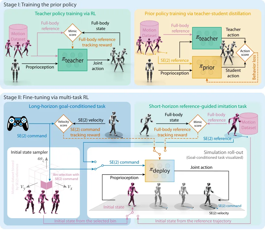
Figure 3 (paper Figure 6): the HuMBLE training pipeline. Three policy instances, two training stages. In Stage I the teacher policy $\pi_{\text{teacher}}$, which tracks a whole-body reference, is distilled into the prior policy $\pi_{\text{prior}}$, which sees only proprioception and the SE(2) command; in Stage II multi-task RL fine-tunes the prior into the final deploy policy $\pi_{\text{deploy}}$, expanding command coverage while preserving the style of the reference data.

The output of the whole pipeline is a policy $\pi_{\text{deploy}}$, parameterized as a single MLP that maps deployment observations directly to joint actions; the inference rate on every platform is 50 Hz. The action $\bm{a}_t$ is multiplied elementwise by a predefined scaling vector and added to nominal joint positions to give desired joint position targets, which a joint-level PD controller tracks. The deployment observation is the concatenation of a proprioceptive part and a steering part:

$$\bm{o}_{\text{deploy}}=(\bm{o}_{\text{prop}},\ \bm{o}_{\text{cmd}}) \tag{1}$$

$$\bm{o}_{\text{prop}}=\big({}_{\mathcal{T}}\bm{v}_{\mathcal{IT}},\ {}_{\mathcal{T}}\bm{\omega}_{\mathcal{IT}},\ {}_{\mathcal{T}}\bm{g}_{\mathcal{I}},\ \bm{q}_{j},\ \dot{\bm{q}}_{j},\ \bm{a}_{t-1}\big) \tag{2}$$

In Eq. (2), ${}_{\mathcal{T}}\bm{v}_{\mathcal{IT}}$ and ${}_{\mathcal{T}}\bm{\omega}_{\mathcal{IT}}$ are the linear and angular velocities measured in the IMU sensor frame $\{\mathcal{T}\}$, ${}_{\mathcal{T}}\bm{g}_{\mathcal{I}}$ is the projected gravity vector in the same frame, $\bm{q}_j$ and $\dot{\bm{q}}_j$ are instantaneous joint positions and velocities, and $\bm{a}_{t-1}$ is the previous action. All six terms are restricted to quantities measurable onboard, which is the precondition for running on hardware. The command observation $\bm{o}_{\text{cmd}}=(\hat{v}_{\text{long}},\ \hat{v}_{\text{lat}},\ \hat{\omega}_{\text{turn}})$ is simply the target longitudinal velocity, lateral velocity, and turning rate.

Note the linear velocity term in Eq. (2): at deployment it depends on the robot's state estimator. On both Atlas machines the estimator is stable enough to give reliable linear velocity feedback indoors and outdoors. On the G1, taken into unstructured outdoor environments, velocity estimates are visibly noisy and drift. The engineering answer was to train an additional policy variant without the linear velocity observation, trading tracking accuracy for stability. The paper gives no quantitative figure for that trade.

Because $\pi_{\text{deploy}}$ is fine-tuned from $\pi_{\text{prior}}$, the two share an identical network architecture and the same observation and action spaces. That constraint runs through the whole paper: the prior must be able to reconstruct whole-body motion consistent with the reference dataset from proprioception and an SE(2) command alone, with no whole-body reference. Partial observability is bridged precisely by teacher-student distillation.

5. Stage I, Part One: The Teacher Policy and Its Reward Engineering

The teacher's observation adds a full-body reference state on top of the deployment observation:

$$\bm{o}_{\text{teacher}}=(\bm{o}_{\text{deploy}},\ \bm{o}_{\text{ref}}) \tag{3}$$

where $\bm{o}_{\text{ref}}=\big({}_{\mathcal{I}}\hat{\bm{r}}^{z}_{\mathcal{IB}},\ {}_{\mathcal{B}}\hat{\bm{v}}_{\mathcal{IB}},\ {}_{\mathcal{B}}\hat{\bm{\omega}}_{\mathcal{IB}},\ {}_{\mathcal{B}}\hat{\bm{g}}_{\mathcal{I}},\ \hat{\bm{q}}_{j}\big)$ are, in order, the reference torso height, reference linear and angular velocities in the torso frame $\{\mathcal{B}\}$, reference projected gravity in $\{\mathcal{B}\}$, and reference joint positions; hatted symbols are imitation targets throughout. The reward has three terms:

$$r_{\text{teacher}}=r_{\text{track}}+r_{\text{reg}}+r_{\text{survival}} \tag{4}$$

$r_{\text{track}}$ drives the robot state onto the reference, $r_{\text{reg}}$ keeps behavior smooth and physically plausible, and $r_{\text{survival}}=c_{\text{survival}}$ is a positive constant paid every step to cancel the incentive to terminate early. After termination, RSI samples and perturbs a new initial condition from the reference data.

The tracking term deserves a close look because it solves two problems at once: inconsistent physical units, and inflated reward on quasi-static motions. For each state variable $i$ (torso linear velocity, torso angular velocity, torso orientation, joint positions) the subterm is an exponential kernel minus a quadratic penalty:

$$r_{\text{track}}=\sum_{i}c_{t,i}\biggl(\kappa_{t}\cdot\exp\Bigl(-\frac{\|\tilde{\bm{e}}_{i}\|}{\lambda_{t}}\Bigr)-\|\tilde{\bm{e}}_{i}\|^{2}\biggr) \tag{9}$$

$\kappa_{t}=5.0$ and $\lambda_{t}=10.0$ are shared across the entire dataset and set the weight of the exponential component against the quadratic penalty. The error itself is normalized by the trajectory $k$ currently being tracked:

$$\tilde{\bm{e}}_{i}=\bm{e}_{i}\oslash\bm{\sigma}^{k}_{i} \tag{10}$$

$\bm{e}_i$ is the raw state error, $\bm{\sigma}^k_i$ is the precomputed standard deviation of state variable $i$ over trajectory $k$, and $\oslash$ is elementwise division. To prevent numerical instability, and to stop quasi-static motions such as standing in place from collecting inflated reward as their standard deviations approach zero, these standard deviations are floored by a user-set minimum $\sigma_{i,\min}$. Reward scale then stays consistent across different physical units and different motion styles, which is what allows one set of weights to train on the whole dataset.

The regularizer $r_{\text{reg}}=\sum_i c_{\text{reg},i}\cdot r_{\text{reg},i}$ contains an action smoothness penalty $\|\bm{a}_t-\bm{a}_{t-1}\|_2$, a joint torque penalty $\|\bm{\tau}_j\|_2$, a slip penalty on contact feet, a foot jerk penalty, and a foot clearance reward. The last of these is more carefully designed than the rest: compute the clearance error $e_{\text{clr},k}=\max(0,{}_{\mathcal{I}}\hat{\bm{r}}^{z}_{\text{clr}}-{}_{\mathcal{I}}\bm{r}^{z}_{\mathcal{IE}_k})$, which penalizes only insufficient swing height and never penalizes swinging higher, then modulate that squared error by the reference foot's horizontal speed:

$$r_{\text{reg},{\text{clr}}}=\sum_{k\in\text{feet}}\exp\Big(-\tanh\big(\lambda_{\text{clr},v}\cdot\|{}_{\mathcal{I}}\hat{\bm{v}}^{xy}_{\mathcal{IE}_{k}}\|\big)\cdot\frac{e^{2}_{\text{clr},k}}{\lambda_{\text{clr},e}}\Big) \tag{12}$$

The $\tanh$ layer does the following: when reference foot speed is high (near the peak of the swing trajectory) the penalty is amplified, and when it is low (the instants of liftoff and touchdown) the influence is minimized. This term is dropped in the goal-conditioned task of stage two, where no reference trajectory, and therefore no reference foot speed, exists.

Training uses PPO with an asymmetric actor-critic. The critic receives privileged environment observations plus a binary "data support" indicator:

$$\bm{o}_{\text{critic}}=(\bm{o}_{\text{deploy}},\ \bm{o}_{\text{ref}},\ \bm{o}_{\text{priv}},\ o_{\text{sup}}) \tag{5}$$

$\bm{o}_{\text{priv}}$ includes torso height, end-effector positions and velocities relative to the torso frame, the current assistive torque level, and generalized end-effector forces. $o_{\text{sup}}\in\{0,1\}$ distinguishes task context: 0 means the steering command lies inside the data support (in-distribution), 1 means an out-of-distribution command. Throughout Stage I it is identically 0, since every command comes straight from the reference data; in Stage II it is set dynamically by environment type. This is a small but consequential design: it gives a single critic the ability to learn a dual value function conditioned on task support.

To absorb the whole motion library without tuning rewards per skill, teacher training reuses the ZEST assistive wrench curriculum: an external force and torque applied to the torso, computed by a model-based PD control law plus a feedforward term compensating nominal torso dynamics:

$$\bm{f}_{\text{assist}}=m\Big({}_{\mathcal{I}}\hat{\dot{\bm{v}}}_{\mathcal{IB}}+k_{p}^{v}({}_{\mathcal{I}}\hat{\bm{r}}_{\mathcal{IB}}-{}_{\mathcal{I}}\bm{r}_{\mathcal{IB}})+k_{d}^{v}({}_{\mathcal{I}}\hat{\bm{v}}_{\mathcal{IB}}-{}_{\mathcal{I}}\bm{v}_{\mathcal{IB}})-{}_{\mathcal{I}}\bm{g}_{\mathcal{I}}\Big) \tag{15a}$$

$$\bm{\tau}_{\text{assist}}={}_{\mathcal{I}}\bm{I}\,{}_{\mathcal{I}}\hat{\dot{\bm{\omega}}}_{\mathcal{IB}}+k_{p}^{\omega}\,{}_{\mathcal{I}}\bm{I}\big({}_{\mathcal{I}}\hat{\bm{\Phi}}_{\mathcal{IB}}\boxminus{}_{\mathcal{I}}\bm{\Phi}_{\mathcal{IB}}\big)+k_{d}^{\omega}\,{}_{\mathcal{I}}\bm{I}({}_{\mathcal{I}}\hat{\bm{\omega}}_{\mathcal{IB}}-{}_{\mathcal{I}}\bm{\omega}_{\mathcal{IB}})+{}_{\mathcal{I}}\bm{\omega}_{\mathcal{IB}}\times({}_{\mathcal{I}}\bm{I}\,{}_{\mathcal{I}}\bm{\omega}_{\mathcal{IB}})-{}_{\mathcal{I}}\bm{r}_{\mathcal{B},\mathrm{com}}\times m\,{}_{\mathcal{I}}\bm{g}_{\mathcal{I}} \tag{15b}$$

The system is approximated as a single rigid body of total mass $m$ and composite rigid-body inertia ${}_{\mathcal{B}}\bm{I}$ (evaluated at the nominal configuration relative to the torso frame), ${}_{\mathcal{I}}\bm{r}_{\mathcal{B},\mathrm{com}}$ is the center-of-mass position relative to the torso frame, and $\boxminus$ is the Lie-group difference on $SO(3)$ (a rotation logarithm map on quaternions, giving the error vector in tangent space). The gains are $(k_p^v,k_d^v)=(0.0,10.0)$ and $(k_p^\omega,k_d^\omega)=(200.0,10.0)$.

Assistance magnitude is scaled by a curriculum gain $\beta\in(0,\beta_{\text{max}})$, and $\beta$ moves up or down under a tracking-similarity metric:

$$s=\frac{1}{\bar{L}_{\mathrm{episode}}}\sum_{t=0}^{\bar{L}_{\mathrm{episode}}}\exp\Big(-\frac{\|\tilde{\bm{e}}_{j,t}\|}{\lambda_{s}}\Big) \tag{16}$$

$\tilde{\bm{e}}_{j,t}$ is the normalized joint position error defined in Eq. (10) and $\lambda_s=10.0$, so $s\in[0,1]$ is a proxy for how well this episode hugged the reference manifold. At episode termination the gain is updated stochastically: increase by $\Delta\beta_{\uparrow}=0.05$ with probability $s$, decrease by $\Delta\beta_{\downarrow}=0.1$ with probability $1-s$. It comes down faster than it goes up, so assistance is withdrawn only after the policy keeps demonstrating tracking capability, while the cap $\beta_{\text{max}}=0.75$ guarantees assistance is always partial. That forces the policy to explore self-sustaining dynamics instead of overfitting to the rewritten physics.

Domain randomization covers Gaussian observation noise, random torso impulses, ground friction, link mass, center-of-mass offsets, joint friction coefficients, and joint zero offsets, with per-platform variation (the high static friction of the Atlas R1 ankle parallel mechanism is covered specifically by joint friction randomization). One scheduling decision here bears directly on style fidelity: training starts on flat ground so the teacher policy first learns the stylistic detail in the data without environmental noise, and terrain randomization is introduced only past the halfway point of teacher training, then kept to the end. The terrain height map (a robot-centric $17\times 11$ grid at 0.1 m spacing, flattened into a vector) is privileged information given only to the critic. As for why it is needed at all: the first time the G1 went to hardware its ankle behavior was too stiff. Simulation showed no problem, but on the real robot any foot touchdown angle deviating from nominal produced frequent stumbling. Adding terrain roughness randomization raised rollout diversity until ankle angles and impact conditions were adequately covered.

6. Stage I, Part Two: DAgger-Style Distillation

Once the teacher is trained, the prior policy is learned by teacher-student distillation, specifically a DAgger variant: rollouts are generated by the student $\bm{\pi}_{\text{prior}}(\bm{o}_{\text{deploy}})$ itself, at each visited state the teacher $\bm{\pi}_{\text{teacher}}(\bm{o}_{\text{teacher}})$ acts as the expert and supplies the action label it would have taken at that same state, and supervised learning minimizes the difference:

$$\bm{\pi}_{\text{prior}}=\arg\min_{\bm{\pi}}E_{\pi}\big\|\bm{\pi}(\bm{o}_{\text{deploy}})-\bm{\pi}_{\text{teacher}}(\bm{o}_{\text{teacher}})\big\| \tag{6}$$

The teacher consumes the whole-body reference; the student is strictly confined to the deployment observation space. That information gap is exactly what forces the prior to internalize, in its own weights, the motion priors and recovery strategies that were previously guided by the teacher's privileged reference observations. The student network is MLP(1024,1024,1024) with ELU activations, wider than the teacher's MLP(1024,512,256); learning rate is fixed at 1e-6, with 4096 parallel environments, batch 98,304 (4096x24), mini-batch 3,072 (32 splits), and a maximum episode length of 150 steps, that is 3 seconds.

7. Stage II: Multi-Task RL Fine-Tuning

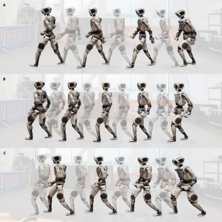
Figure 4 (paper Figure 2): stroboscopic comparison of Atlas R1 under a constant forward velocity command. Every frame is caught at the swing-phase to ground-contact transition, to show whether arm swing, heel strike, and knee lock are synchronized. (A) the HuMBLE policy, (B) an MPC controller, (C) a Tabula Rasa RL policy; all three start from a standing configuration.

The Stage I prior is highly faithful for commands inside the data distribution but struggles with out-of-distribution velocity commands. Diagonal translation combined with fast turning is the canonical case: reachable by a joystick, rare in human gait. Stage II has to extend command coverage to the operating range that actually matters, and improve robustness along the way. The most direct approach is fine-tuning against a reward that "tracks any velocity command", and that usually produces style collapse: to track commands accurately the policy gives up the natural motion patterns learned in Stage I.

HuMBLE's answer is to write Stage II as a multi-task RL problem and run the two task groups simultaneously across parallel simulation environments:

$$r_{\text{fine-tune}}=\begin{cases}r_{\text{ref}} & \text{if env}\in\mathbb{E}_{\text{ref}}\\ r_{\text{goal}} & \text{if env}\in\mathbb{E}_{\text{goal}}\end{cases} \tag{7}$$

The $\mathbb{E}_{\text{ref}}$ group is a short-horizon reference-guided imitation task: it keeps tracking the reference dataset and acts as the style-preserving regularizer, conceptually a kind of style-constrained experience replay. The $\mathbb{E}_{\text{goal}}$ group is a long-horizon goal-conditioned task: it optimizes purely for robustly tracking randomly sampled velocity commands and involves no reference-tracking objective at all. In the nominal configuration the two groups split the environments evenly (50:50).

The two groups have very different episode lengths, and not by accident. The reference-guided group reuses the teacher reward $r_{\text{ref}}=r_{\text{teacher}}$ (Eq. 4) and RSI initialization, with the single difference that the policy sees $\bm{o}_{\text{deploy}}$ but not $\bm{o}_{\text{ref}}$. Under that partial observability, small tracking errors are unavoidable even for a policy distilled to reconstruct the reference; and because it cannot observe the reference, once it drifts too far it cannot produce effective corrections, so errors accumulate over long episodes until the policy ends up where the reference-tracking reward carries no information. This group is therefore deliberately set to 150 steps (3 seconds), concentrating the reinforcement signal on local style preservation and keeping long-horizon accumulated drift from steering the optimization.

The goal-conditioned group computes reward without any reference trajectory:

$$r_{\text{goal}}=r_{\text{cmd}}+r_{\text{reg}}+r_{\text{survival}} \tag{8}$$

$$r_{\text{cmd}}=\sum_{i}c_{\text{cmd},i}\cdot\exp\Big(-\frac{\|\bm{e}_{i}\|^{2}}{\lambda_{\text{cmd},i}}\Big) \tag{14}$$

Eq. (14) has two error branches: linear velocity command tracking $\bm{e}_v=(\hat{v}_{\text{long}},\hat{v}_{\text{lat}})-(v_{\text{long}},v_{\text{lat}})\in\mathbb{R}^2$, and turning rate command tracking $\bm{e}_{\text{turn}}=\hat{\omega}_{\text{turn}}-\omega_{\text{turn}}\in\mathbb{R}$. Weights $c_{\text{cmd},i}$ and exponential scales $\lambda_{\text{cmd},i}$ are given in supplementary Table S6. The regularizer and survival terms are identical to the teacher's, and termination conditions are shared (for example, termination on excessive contact force). Episodes in this group run 400 steps (8 seconds) and allow commands to be resampled within an episode, which exposes the policy to transitions between commands; beyond the standard termination conditions, the episode also ends when the robot falls into an unrecoverable state and can no longer track commands.

Goal-conditioned rollouts are initialized by a dedicated scheme the authors call goal-conditioned reference state initialization (GC-RSI): take the target velocity command and retrieve a frame from the dataset whose annotated command is nearby. For fast retrieval, reference states are pre-binned by annotated command into a lookup table; given a query command, a frame is sampled from the corresponding bin, a candidate state is picked at random inside a time window centered on that frame, and a small perturbation is applied to produce the initial state.

This mechanism buys two things. First, it anchors fine-tuning to states that still lie within the support of the learned behavior prior: $\bm{\pi}_{\text{prior}}$ already knows how to control motions drawn from the data distribution, so starting from a reference state whose annotated command is close to the sampled command lets the policy lean on its existing prior at the beginning of every episode. It does not immediately drift into out-of-distribution states and does not develop an isolated behavior mode unrelated to the reference motions, so command coverage expands gradually while style and dynamic structure survive. Second, it avoids a severe mismatch between command and initial state, which is especially damaging at large commands: forcing the robot to accelerate hard from a mismatched posture tends to terminate the episode before any meaningful learning signal is produced.

Finally, the optimization details of fine-tuning, several of which exist purely to avoid washing out the style that was already learned. Cold-starting PPO from the distilled prior is problematic: a randomly initialized critic gives noisy, unreliable value estimates, and an actor updated against those estimates erodes the stylistic detail from Stage I quickly. Fine-tuning therefore begins by loading both the $\bm{\pi}_{\text{prior}}$ policy network and the critic $V_{\text{teacher}}$ from teacher training. But $V_{\text{teacher}}$ approximates the value function of the teacher policy, not of the prior, so it must be adapted first: 5000 iterations of critic-only warm-up on the reference-guided task ($V_{\text{teacher}}\rightarrow V_{\text{prior}}$, policy frozen), then the full multi-task RL that jointly trains $\bm{\pi}_{\text{prior}}\rightarrow\bm{\pi}_{\text{deploy}}$ and $V_{\text{prior}}\rightarrow V_{\text{deploy}}$.

Because the two tasks have different reward functions, the critic must predict returns under each. This is where $o_{\text{sup}}$ from Eq. (5) earns its place: it is provided only to the critic, as the context signal identifying the current task domain. It is 0 in short-horizon reference-guided environments and 1 in long-horizon goal-conditioned environments, so the critic learns a dual value function conditioned on task support. Advantage estimates for the two environment groups are also normalized separately (the same treatment as RobotKeyframing) to absorb the scale difference between the two reward functions. Beyond that, the learning rate drops to a fixed 1e-6, the policy entropy coefficient is squeezed to 0.001 (0.0015 during the teacher stage), the initial action noise standard deviation is only 0.16 (1.0 during the teacher stage), and the GAE $\lambda$ moves from 0.95 to 1.0. All of it is small-step updating configured to protect style.

flowchart TB
    MOCAP["Vicon 120 Hz capture
actor 178 cm"] --> RET["Two-stage retarget
proxy skeleton then robot"]
    RET --> SCALE["0.8x spatial scale
time warp factor 1/sqrt(0.8)"]
    SCALE --> ANN["Per-frame SE(2) command annotation
finite diff + lowpass + backward shift"]
    ANN --> DS[("Dataset N=528214 frames
about 3 h, sagittal mirrored")]
    DS --> TEA["Stage I teacher RL with PPO
o_teacher = o_deploy + o_ref
r_track + r_reg + r_survival
assistive wrench curriculum"]
    TEA --> DIST["Teacher-student distillation
DAgger variant
student rollouts, teacher labels"]
    DIST --> PRIOR["pi_prior MLP 1024x3
proprioception + SE(2) command only"]
    PRIOR --> WARM["Critic warm start 5000 iters
V_teacher to V_prior, policy frozen"]
    WARM --> MT["Stage II multi-task RL
PPO lr 1e-6, entropy 0.001"]
    DS --> EREF["E_ref short horizon 150 steps
r_ref = r_teacher
style regularizer, o_sup = 0"]
    DS --> GCRSI["GC-RSI init
command-binned lookup table"]
    GCRSI --> EGOAL["E_goal long horizon 400 steps
r_goal = r_cmd + r_reg + r_survival
command resampled in episode, o_sup = 1"]
    EREF -->|50 percent of envs| MT
    EGOAL -->|50 percent of envs| MT
    MT --> DEP["pi_deploy at 50 Hz
1.1 ms on Jetson AGX Orin CPU"]
    DEP --> R1["Atlas R1
push recovery up to 1400 N"]
    DEP --> D1["Atlas D1
backward, circle, sidestep"]
    DEP --> G1["Unitree G1
walk to sprint transition"]
    DEP --> HIGH["Hierarchical stacks
joystick / waypoint nav / box parkour MoE 10 Hz"]

Figure 5: the full HuMBLE flow, drawn from the paper's method. The left data path (capture, two-stage retarget, scaling and temporal warp, command annotation, mirroring) produces the single dataset that simultaneously feeds the Stage I teacher RL, the Stage II reference-guided group, and the GC-RSI lookup table; the right side shows how the three policy instances hand off to one another, and the three hardware platforms plus hierarchical applications the result lands on.

8. Experiment One: Data Fidelity, and How Much the Student Loses

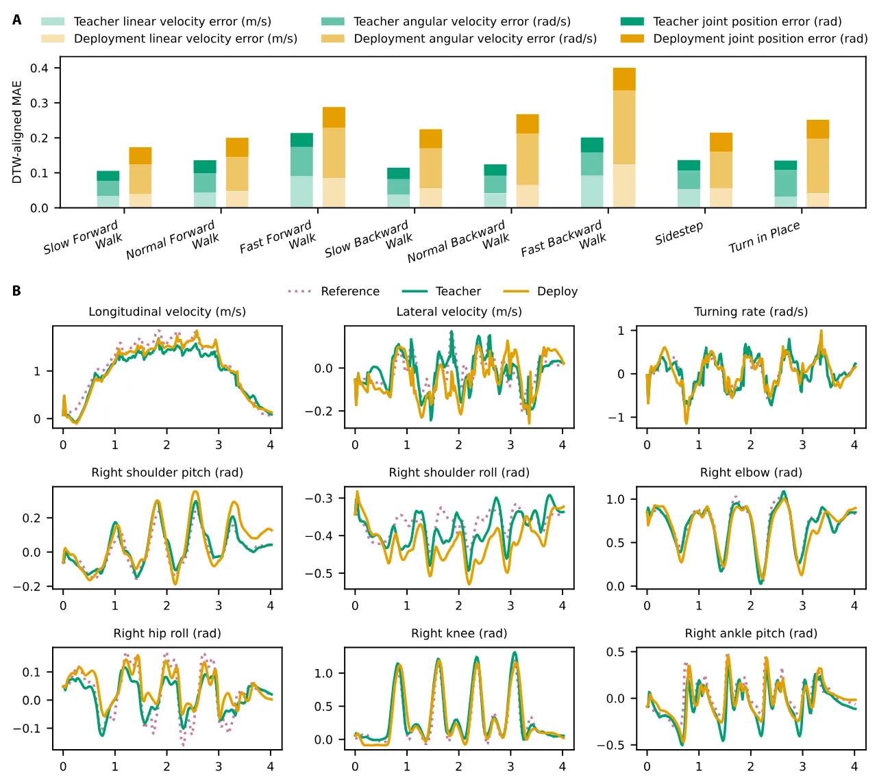
Figure 6 (paper Figure 3): data fidelity analysis. (A) Mean absolute error of torso linear velocity, angular velocity, and joint positions relative to the reference motion, teacher policy versus final deploy policy; each bar decomposes cumulative tracking error into the three physical units. (B) Fast Forward Walk: reference motion, whole-body-reference-conditioned teacher policy, and command-conditioned deploy policy compared. These curves are raw time series with no DTW applied; the horizontal axis is seconds, showing SE(2) torso velocities and selected joint angles chosen to expose human-like traits (arm swing, hip sway, knee extension, heel-to-toe rolling).

Style quality is subjective and hard to measure directly, so the paper quantifies a proxy: fidelity to the retargeted human motion data. The proxy is defensible, because the final deploy policy receives no whole-body reference and must reconstruct whole-body behavior from proprioception and an SE(2) velocity command alone. Its deviation from the reference trajectory therefore measures directly how much of the motion patterns in the dataset it managed to preserve.

The choice of comparison is also deliberate. Alongside the deploy policy, the paper uses the teacher policy as an upper bound. The teacher is trained in a motion imitation framework and conditioned on the full-body reference, so it gives the bound of a "dynamically feasible reference implementation". That step is necessary: kinematic references often carry non-physical artifacts introduced by the retargeting process, and using the raw reference as the bound would unfairly penalize the deploy policy.

Evaluation is in simulation, on the Unitree G1 deploy policy, across eight canonical motions drawn from the reference data: forward walking at three speeds (slow, normal, fast), backward walking at three speeds, turning in place, and sidestepping. For each trajectory the SE(2) velocity command annotated in the reference data is fed to the deploy policy as the steering command and the resulting robot trajectory is collected. Because small temporal misalignments between the reference trajectory and the simulation rollout would artificially inflate tracking error, the two are aligned by dynamic time warping (DTW) before comparison: distance is computed over the concatenated vector of torso linear velocity, angular velocity, and joint positions, with sample points paired under a strictly monotonic time-index constraint. Across the full scenario set DTW introduces a mean temporal displacement of only 68.7 ms, indicating that alignment absorbed phase differences without distorting trajectory shape.

The results: the deploy policy's DTW-aligned MAE is 0.058 m/s for torso linear velocity, 0.127 rad/s for torso angular velocity, and 0.055 rad for joint positions; the teacher policy gives 0.048 m/s, 0.055 rad/s, and 0.033 rad. In other words, tracking error on these three components is larger for the deploy policy by 20.83%, 130.31%, and 67.58%. The paper explains the gap on two levels: the teacher has direct access to the whole-body reference state while the deploy policy must reconstruct it from partial observations; and the deploy policy additionally went through a command-conditioned fine-tuning stage, which by construction introduces deviation from the reference.

Absolute values alone are hard to judge, so the paper normalizes error by the standard deviation of the reference trajectories themselves: $\sigma_{\bm{v}}=0.390\ \mathrm{m/s}$, $\sigma_{\bm{\omega}}=0.491\ \mathrm{rad/s}$, $\sigma_{j}=0.300\ \mathrm{rad}$, which puts the deploy policy at 0.149$\sigma_{\bm{v}}$, 0.257$\sigma_{\bm{\omega}}$, 0.184$\sigma_j$. With no visibility of the whole-body reference at all, its deviation stays within a quarter of the reference distribution's own variability. Supplementary Table S1 gives the per-motion breakdown:

Motion clip (Unitree G1, simulation)	Linear vel. MAE Teacher	Linear vel. MAE Deploy	Angular vel. MAE Teacher	Angular vel. MAE Deploy	Joint pos. MAE Teacher	Joint pos. MAE Deploy
Slow Forward Walk	0.0341	0.0388	0.0421	0.0852	0.0294	0.0491
Normal Forward Walk	0.0441	0.0472	0.0541	0.0979	0.0376	0.0547
Fast Forward Walk	0.0895	0.0847	0.0841	0.1438	0.0402	0.0598
Slow Backward Walk	0.0383	0.0550	0.0435	0.1149	0.0326	0.0549
Normal Backward Walk	0.0418	0.0643	0.0496	0.1478	0.0328	0.0555
Fast Backward Walk	0.0916	0.1233	0.0665	0.2112	0.0427	0.0657
Sidestep	0.0537	0.0546	0.0523	0.1054	0.0304	0.0549
Turn in Place	0.0322	0.0418	0.0753	0.1555	0.0275	0.0544
Mean	0.0480	0.0588	0.0551	0.1269	0.0330	0.0553

Table 1: full values from the paper's Table S1, in units of m/s, rad/s, and rad respectively. Mean DTW temporal warping is 10.05 ms for the teacher and 68.73 ms for the deploy policy.

Several things in this table carry more information than the means. First, angular velocity is the component the student loses most on (0.0551 to 0.1269, more than double), and it does not come close to the teacher on a single one of the eight clips: turning and orientation regulation are the hardest parts of an SE(2) command to reconstruct from command plus proprioception alone. Second, Fast Forward Walk is the only clip where the deploy policy's linear velocity MAE is actually lower than the teacher's (0.0847 versus 0.0895), which says that in a data-dense high-speed forward regime, the stage-two command-tracking fine-tune can push linear velocity below what pure imitation achieves. Third, backward walking degrades systematically more than forward walking (Slow Backward linear velocity 0.0383 to 0.0550, Fast Backward 0.0916 to 0.1233); backward locomotion relies more on vision and exteroception than forward locomotion, so removing them and leaving only proprioception costs more. Fourth, on Sidestep the deploy policy's linear velocity nearly matches the teacher (0.0546 versus 0.0537) but its mean temporal warping reaches 169.4 ms, the largest of any clip: lateral motion is the hardest to phase-align, and a small absolute error does not mean the temporal structure is right.

Figure 3B supplies the temporal dimension: with no DTW, looking directly at raw time series, the deploy policy follows the teacher's and the reference's phase and amplitude trends on linear velocity, angular velocity, and the representative joints (shoulder and elbow for arm swing, hip roll for lateral balance and torso regulation, knee for stance-leg extension, ankle pitch for touchdown and heel-to-toe rolling). Given that it receives only proprioception and one SE(2) command, this says it preserved not just the commanded torso motion but the upper- and lower-limb coordination patterns in the data.

9. Experiment Two: Command Coverage, Rise Time, and Push Robustness

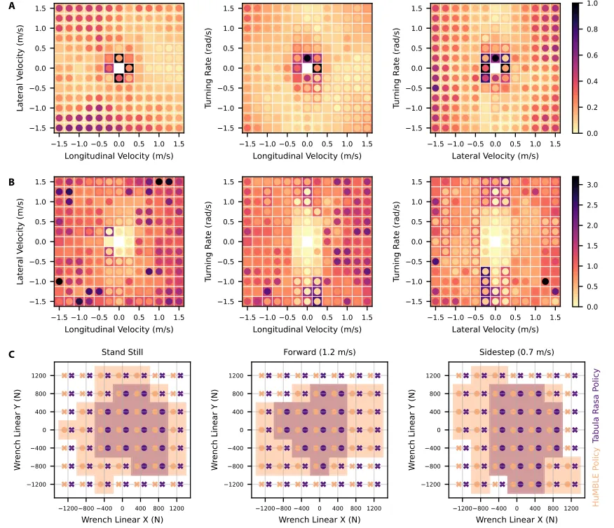
Figure 7 (paper Figure 4): quantitative performance analysis on Atlas R1, comparing the HuMBLE and Tabula Rasa policies. (A) Steady-state relative command-tracking error: the SE(2) command space is visualized as three 2D slices, zeroing from left to right $\omega_{\text{turn}}$, $v_{\text{lat}}$, and $v_{\text{long}}$; in each cell the outer square is the Tabula Rasa baseline and the inner circle is HuMBLE, with lighter colors meaning better. (B) Rise time in seconds, visualized the same way. (C) Push robustness: planar pushes of varying magnitude in three locomotion scenarios; shaded regions approximate the successful recovery envelopes of HuMBLE (orange) and Tabula Rasa (purple), circles mark successful recovery and crosses mark falls.

The control group is a Tabula Rasa RL policy: identical observation and action spaces to the final deploy policy, also mapping proprioception plus SE(2) commands straight to joint actions, but using no human motion data at all and shaping emergent gaits purely by hand-crafted reward. Its regularizer is consequently far more complex than HuMBLE's (torso upright, roll, and pitch penalties, deviation-from-nominal-configuration penalty, soft joint limits, foot acceleration and jerk penalties, slip penalty, a yaw limit on feet relative to the torso, a ground-contact term, torque and joint acceleration penalties, plus a foot clearance profile that encourages swing-leg air time and a maximum swing height of 0.15 m). Its curriculum is not the assistive wrench, which requires a reference trajectory it does not have, but a velocity command sampling range that adaptively expands or contracts with tracking fidelity. PPO hyperparameters match the HuMBLE teacher stage, domain randomization is identical, and termination conditions align with HuMBLE's goal-conditioned task. The authors state plainly that this baseline "may not represent a globally optimal control design"; its role is a representative, deployable, command-tracking-robust reference under exactly the same observation, action, and domain randomization specification.

The evaluation protocol borrows from classical step-response analysis: each command is applied as a step input, steady state is taken as the torso velocity 3.0 s after the step, and rise time is defined as the duration from step onset to first reaching 90% of the steady-state torso velocity; relative command-tracking error is steady-state error divided by command magnitude. All policies are trained and evaluated in Isaac Lab, with responsiveness, command coverage, and robustness cross-validated in a MuJoCo-based simulation pipeline. That pipeline is a hardware-validated high-fidelity proxy and reflects real deployment constraints.

The conclusion from Figure 4A: across most of the evaluated SE(2) command space, HuMBLE's relative tracking error is comparable to the Tabula Rasa baseline; the most significant errors appear in command regions underrepresented or absent in the motion data, such as fast diagonal walking. Conversely, on near-zero velocity commands HuMBLE outperforms the baseline, which the authors attribute to the slow-shuffling references in the dataset. For "small but non-zero" locomotion commands, task-reward optimization struggles to discover a suitable gait on its own; the motion prior hands it over.

On responsiveness (Figure 4B), both policies show longer rise times as command magnitude grows; the Tabula Rasa baseline typically reaches large commands faster, while HuMBLE gives smoother, more gradual responses in the high-speed regime. That pattern matches the acceleration profiles inherent in the human motion data, and it is the direct expression of the trade-off between naturalistic transitions and aggressive command tracking.

The robustness test pushes the torso with planar forces: force is applied in continuous 0.2 s pulses, timed after the policy reaches steady-state velocity, with the target command held constant throughout the test; scenarios are standing still, forward walking, and sidestepping. A fall is declared when torso pitch or roll tilt exceeds 30 degrees, or when torso height drops below 40% of nominal standing height (the Atlas R1 values). HuMBLE withstands pushes up to 1400 N along the principal directions on Atlas R1. More interesting is that push resistance shows a directional dependence tightly aligned with gait kinematics: during forward walking, longitudinal resistance exceeds lateral resistance, mainly from sagittal-plane leg swing and the effective support polygon formed during forward motion; during sidestepping the stance is wider, lateral stability rises and longitudinal stability falls.

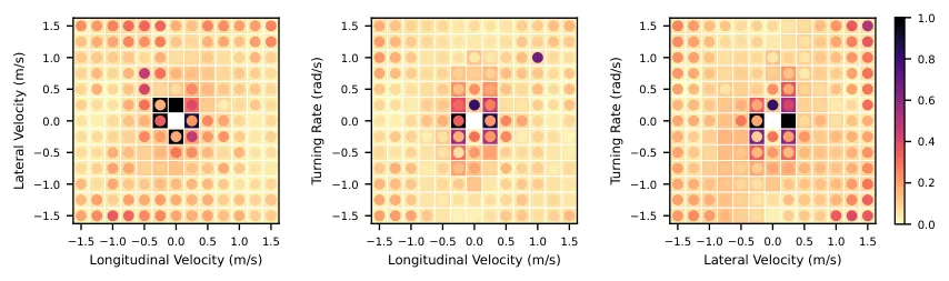
Figure 8 (part of paper Figure S2): the same quantitative evaluation on Atlas D1, steady-state relative command-tracking error and rise-time heatmaps, sliced the same way as Figure 4 (left to right $\omega_{\text{turn}}=0$, $v_{\text{lat}}=0$, $v_{\text{long}}=0$). The supplementary material also provides Figure S3 for the Unitree G1, noting that because spatial and temporal scaling was applied during retargeting, the command range used for G1 evaluation differs from the two Atlas platforms.

The exact evaluation metrics differ across the three platforms, but the trend is the same: HuMBLE policies match the Tabula Rasa baselines on command-tracking accuracy, responsiveness, and disturbance robustness, at the cost of slightly longer rise times in the high-speed regime. The paper attributes that directly to the naturalistic acceleration profiles learned from human reference data rather than to a capability deficit.

The qualitative comparison in Figure 2 says something the heatmaps cannot. Against the MPC baseline (Boston Dynamics' default controller, footstep planning tracked by model predictive control), HuMBLE shows synchronized arm swing, knee extension near stance, hip motion used to regulate torso orientation, a heel-strike-like contact transition, and heel-to-toe rolling of the stance foot, while the MPC keeps limbs nearly fixed relative to the torso and looks more strictly periodic. Against Tabula Rasa, it shows stronger upper-lower body spatiotemporal coordination, clear knee locking, and prominent heel-to-toe rolling during contact, which produces smoother momentum transfer and quieter steps. On Atlas D1, despite non-human foot morphology, the policy retains heel-to-toe rolling consistent with the human prior. Gait style also adapts across commanded speeds: a flatter shuffling gait at low speed, transitioning toward pronounced heel strike and toe-off as commanded speed increases.

10. Experiment Three: Sim-to-Real and Onboard Real-Time Performance

Transfer consistency is measured by running the same representative commands through the step-response protocol in simulation and on hardware: forward walking, backward walking, sidestepping, turning in place, and forward circling, each at slow, normal, and fast settings. Every rollout starts from the robot standing still at zero command, then a rectangular pulse command is applied, held, and returned to zero. Both whole-rollout MAE (which captures differences in the step transient) and steady-state error are reported; the linear error is the larger of the longitudinal and lateral tracking errors. The Atlas R1 results follow (from the paper's Table 1):

Command $(v_{\text{long}},v_{\text{lat}},\omega_{\text{turn}})$	Steady-state error Sim	Steady-state error Real	MAE Sim	MAE Real
Forward walk (0.4, 0.0, 0.0)	(0.08, 0.02)	(0.12, 0.03)	(0.10, 0.10)	(0.11, 0.10)
Forward walk (1.2, 0.0, 0.0)	(0.03, 0.02)	(0.06, 0.07)	(0.10, 0.15)	(0.10, 0.18)
Forward walk (2.0, 0.0, 0.0)	(0.13, 0.11)	(0.20, 0.06)	(0.15, 0.13)	(0.18, 0.16)
Backward walk (-0.9, 0.0, 0.0)	(0.10, 0.02)	(0.20, 0.10)	(0.11, 0.12)	(0.14, 0.16)
Sidestep (0.0, -1.0, 0.0)	(0.27, 0.04)	(0.25, 0.09)	(0.19, 0.08)	(0.21, 0.11)
Turn in place (0.0, 0.0, 2.0)	(0.02, 0.27)	(0.06, 0.34)	(0.10, 0.22)	(0.10, 0.25)
Turn in place (0.0, 0.0, -3.0)	(0.07, 0.53)	(0.05, 0.60)	(0.11, 0.34)	(0.13, 0.39)
Forward circle (1.0, 0.0, -1.5)	(0.08, 0.25)	(0.11, 0.33)	(0.10, 0.18)	(0.13, 0.24)

Table 2: sim-to-real comparison on Atlas R1 (from the paper's Table 1). Each cell is (linear error m/s, angular error rad/s). The full table in the paper also contains rows for (-0.3,0,0), (-1.5,0,0), (0,+/-0.7,0), (0,+/-1.0,0), (0,0,+/-1.0), (0,0,+/-2.0), (0,0,3.0), (1.0,0,+/-1.0), and (1.0,0,1.5); the corresponding Atlas D1 and Unitree G1 results are in Table S2.

How to read this: simulation and hardware tracking errors agree closely, and for the large majority of commands the difference stays within 0.05 m/s of linear error and 0.10 rad/s of angular error. Error grows as commands get more aggressive, most extremely at the 3.0 rad/s in-place turn, where steady-state angular error already reaches 0.47 to 0.53 rad/s in simulation and 0.42 to 0.60 rad/s on hardware. The key point is that this upward trend appears on both sides, so it is not a transfer failure but the task itself getting harder at the edge of the command space. The paper does concede that in the most aggressive region the sim-to-real gap widens slightly; the forward circle at 1.5 rad/s, with MAE going from 0.10/0.18 in simulation to 0.13/0.24 on hardware, is one such example.

On real-time performance: because the policy is just a lightweight MLP, it runs onboard in real time on all three platforms. On the Unitree G1, using ONNX Runtime on the robot's NVIDIA Jetson AGX Orin CPU, mean single-inference latency measures 1.1 ms against a 50 Hz control rate, that is a 20 ms period budget. Inference latencies on the two Boston Dynamics machines are withheld under proprietary agreement. During joystick deployment the steering input is additionally processed into bounded rates of change; the trade the authors make is a little responsiveness for a smoother driving feel.

11. Ablations: What Each of the Three Design Choices Contributes

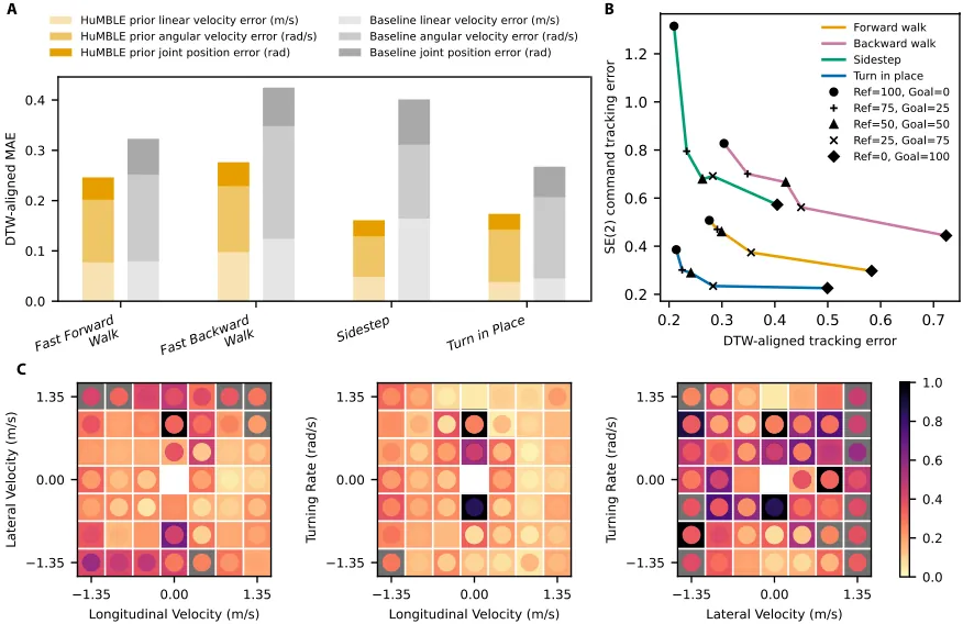
Figure 9 (paper Figure 5): the three ablations. (A) The role of teacher-student distillation: the Stage I distilled prior (orange) versus a single-stage RL baseline trained directly as a command-conditioned policy (gray); stacked bars are component-wise MAE after DTW alignment. (B) The effect of multi-task RL: environment allocation ratio swept on four canonical modalities, evaluating data fidelity and command tracking together. (C) The impact of RL fine-tuning: steady-state relative command-tracking error of the final deploy policy (inner circle) against its initialization source, the Stage I prior (outer square); gray cells mark commands where the prior cannot track robustly and the robot falls.

The first ablation asks whether teacher-student distillation is genuinely necessary to learn a reliable command-conditioned prior, or whether the prior could be trained directly in the deployment observation space with imitation rewards from the reference motions. The comparison $\bm{\pi}_{\text{baseline}}(\bm{o}_{\text{deploy}})$ uses the same deployment observation space and the same tracking reward $r_{\text{teacher}}$, that is, it is forced to reconstruct reference trajectories from proprioception and steering commands alone; to control variables it reuses exactly the asymmetric critic architecture and hyperparameters of the teacher training stage. Evaluation is in Unitree G1 simulation with the same metrics as the fidelity analysis.

Comparison (MAE increase relative to the HuMBLE prior)	Linear vel.	Angular vel.	Joint pos.	Qualitative outcome
Single-stage baseline, summed over Fast Forward Walk / Fast Backward Walk / Turn in Place	+16.36%	+54.85%	+70.87%	Reproduces the reference motions, but error is uniformly higher
Single-stage baseline, Sidestep	+240.87%	+80.54%	+186.34%	Takes a few steps then settles into a near-standing pose and stops responding to turning commands
Stage II ratio 0:100 (purely goal-conditioned)	Fidelity lost rapidly			Torso writhing during forward and backward walking, arm swing inconsistent with the reference
Stage II ratio 100:0 (purely reference-guided)	Insufficient command coverage			Cannot execute sidestep commands and falls (lateral commands are already sparse in the data)

Table 3: key numbers and qualitative observations from the three ablations in Section 5 of the paper. The first two rows come from Figure 5A, the last two from the extreme ratios of Figure 5B.

The gap is largest on sidestepping, which is precisely the behavior that demands the most coordination: lateral balance plus accurate whole-body timing. There the single-stage baseline does not merely track poorly, it fails to reconstruct the behavior at all. After a few steps it lands in a near-standing pose and stops reacting to turning commands. The authors' conclusion is that single-stage partially observable imitation recovers some motion modalities but is unreliable at preserving the full behavioral diversity in the data; the value of teacher-student distillation is that it decouples two hard problems. The teacher first learns a dynamically feasible realization of the whole-body reference in simulation, then the student distills that behavior into the deployment observation space.

The second ablation sweeps the Stage II environment allocation ratio: starting from the same Stage I prior, fine-tune at 0:100, 25:75, 50:50, 75:25, and 100:0 (the first number is the share of reference-guided environments), then evaluate reference-tracking fidelity and command tracking together. On the fidelity side the policy is driven by the time-varying SE(2) command annotated from the corresponding reference motion, reporting DTW-aligned whole-body tracking error on the same benchmark clips (Fast Forward Walk, Fast Backward Walk, Sidestep, Turn in Place); on the command-tracking side it is driven by constant commands per modality, forward walk $(1.35,0,0)$, backward walk $(-1.35,0,0)$, sidestep $(0,1.35,0)$, turn in place $(0,0,1.7)$, reporting mean velocity tracking error. Together the curves trace the Pareto trade-off induced by the multi-task fine-tuning objective: more reference-guided environments stay closer to the data, more goal-conditioned environments track commands better. Each extreme exposes one failure mode (Table 3), and the nominal 50:50 is a usable interior point. The authors frame this ratio as an interpretable hyperparameter to be tuned for the deployment behavior you want.

The third ablation puts the Stage I prior and the final deploy policy on the same command grid and compares steady-state relative tracking error (Unitree G1, reusing the step-response protocol of the main experiments). The prior holds reasonable tracking in regions where the data distribution is dense, but degrades quickly where reference data is sparse or absent: in several high-speed command regions it cannot respond robustly to turning commands, showing dynamic instability and frequent falls. The most pronounced case is lateral motion combined with yaw, exactly the sparsest region of the dataset in Figure 7, where falls are unavoidable. After fine-tuning, the deploy policy has uniformly lower tracking error across the entire operating space, greatly expanded command coverage, and not a single fall across all test cases, with no collapse into unnatural gaits. The verdict from this ablation is blunt: teacher-student distillation alone does not reach the responsiveness and command coverage real deployment requires, and the Stage II multi-task RL fine-tune is what makes this humanoid locomotion policy robust on general locomotion tasks.

12. Hierarchical Applications: HuMBLE as a Low-Level Module

Three scenarios show the policy being driven by something above it: operator control with a joystick supplying SE(2) velocity targets directly; autonomous navigation with obstacle and hazard avoidance, planning paths to waypoints in a warehouse environment; and box parkour, combining HuMBLE with separately learned climbing behaviors. In joystick deployment the policy is stable and responsive to a broad command range in both lab and real-world settings, and shows smooth emergent gait transitions: shuffling steps at low commanded velocity, standard-pace walking with nominal strides at mid range, and sprinting with large strides and distinct flight phases at high velocity.

The box parkour implementation detail is in supplementary Section S7, and it shows how the hierarchical framework can be assembled. The high-level policy is perceptive, emitting SE(2) velocity commands $(v_{\text{long}},v_{\text{lat}},\omega_{\text{turn}})$ plus a set of gating weights at 10 Hz; the low level is three frozen pretrained experts, the HuMBLE policy, a box-up policy, and a box-down policy, each emitting joint position targets at 50 Hz. Velocity commands are low-pass filtered first to prevent jumps, then distributed in whatever representation each expert needs: HuMBLE receives velocity commands directly, while the two climbing experts receive SE(2) pose waypoints obtained by integrating the velocity command. The three experts' outputs are averaged with the normalized gating weights to produce the final action. Only the high level is perceptive; the low-level experts are not. The Unitree G1 completes multiple long-horizon navigation tasks in environments with one and two boxes, deployed zero-shot on hardware, with the transitions and concatenations between walking, box-up, and box-down selected and blended online by the high level.

The way the two climbing experts are trained both overlaps with and departs from the HuMBLE teacher, and the difference is worth recording: they also use PPO for reference-guided imitation following ZEST, but the command is defined as an SE(2) pose waypoint rather than a velocity (at each timestep an expected future pose is defined by the reference motion and its mirror over a 0.5 s look-ahead horizon, expressed in the robot's torso heading frame, with Gaussian noise added to the waypoint command to absorb high-level planner error); and they do not consume whole-body reference states, so they need no distillation to deploy directly and generalize better to unseen conditions. Their critic's privileged information is replaced by a tracking score and a task phase variable that ramps from 0 to 1 along the reference trajectory. The high-level policy is trained in two stages: first only the three primitive tasks (walk, box-up, box-down) sampled with equal probability, then three composite tasks are added (walk into box-up, box-up into box-down, box-down into walk) sampled at half the primitive probability. It observes proprioception, SE(2) goal pose commands, and a local height scan; its critic additionally receives torso height and, for climbing motions only, the error of torso height relative to the reference.

13. Limitations

The authors state three. First, results cover flat terrain only. Extension to mild terrain roughness is immediate with more thorough domain randomization, but more general locomotion scenarios such as stair climbing, whole-body climbing, and stepping over obstacles remain open: they require both a new set of human motion references able to capture these agile behaviors and a policy conditioned on terrain observations, which introduces exteroceptive sensing at deployment.

Second, the command annotation only fits SE(2). The approach here is post-hoc: after collection, estimate the actor's locomotion intent and label each frame with an SE(2) velocity command. That is straightforward for SE(2) because the command can be computed from the reference trajectory itself, but it does not extend to more complex steering modalities. Higher-level semantic annotations such as natural language would probably require manual labeling or more advanced captioning techniques.

Third, network capacity and scalability were not rigorously analyzed. The authors deliberately chose a simple MLP with a modest parameter count to keep deployment compute and memory low, and the results show this compact architecture is sufficient to internalize and reconstruct whole-body behavior from velocity commands, capturing the distribution of a dataset with N=528,214 frames (about three hours). But how parameter count affects performance, where the capacity limit of this architecture lies, and under what boundary conditions the policy starts failing to capture the data distribution all remain open questions.

The following are my own judgments after reading the main text and the supplementary material. First, fidelity is quantified on the G1 only. All eight canonical clips and their DTW-MAE come from Unitree G1 simulation; Atlas R1 and D1 get heatmaps (Figure 4, Figure S2) and sim-to-real tables (Table 1, Table S2), which measure command tracking rather than style fidelity. The claim that all three platforms preserve human style therefore holds, under a single yardstick, for one robot.

Second, using MAE as a style proxy has a price. The paper itself concedes that style quality is inherently subjective and hard to measure directly, hence fidelity to retargeted data as a proxy. But low MAE does not equal natural appearance: in Table S1 the deploy policy's Sidestep linear velocity error (0.0546) nearly matches the teacher (0.0537), while its temporal warping is the largest in the table at 169.4 ms, meaning numbers can be close while temporal structure is far apart. There is no human subjective evaluation anywhere in the paper (no user study, no preference ranking), and human-legible gait is precisely what this paper sells.

Third, the strength of "comparable to the baseline" is bounded by how well the baseline was tuned. The Tabula Rasa baseline is the authors' own implementation, and the paper's own words are that it "may not represent a globally optimal control design" and that performance varies with alternative RL formulations. The command-tracking and push-envelope comparisons are therefore an internal control, not a comparison against externally published methods.

Fourth, robustness is reported only as a binary success/failure envelope. The push test tells you whether the robot avoids falling, with no recovery time, no trajectory deviation during recovery, and no energy cost. The 1400 N number therefore locates the envelope boundary but says nothing about behavior quality near that boundary. Separately, outdoor G1 deployment depends on the state estimator for the linear velocity observation, and the authors trained an extra policy variant without it, stating plainly that it reduces velocity tracking accuracy, but that accuracy loss is never quantified.

14. Conclusion and Outlook

The skeleton of this paper is a division of labor: style belongs to stage one, coverage belongs to stage two. Stage one uses a privileged teacher with access to the whole-body reference to learn, as a dynamically feasible realization, the things three hours of human motion data contain that reward engineering struggles to produce: synchronized arm swing, knee locking in the stance leg, the heel-strike to toe-roll contact transition, and speed-dependent gait switching. DAgger-style distillation then compresses that into an MLP seeing only proprioception and an SE(2) command. Stage two fine-tunes it with a group of short-horizon reference-guided environments and a group of long-horizon goal-conditioned environments running together, the former as style regularizer and the latter expanding command coverage, with GC-RSI anchoring every rollout's start inside the prior's support, $o_{\text{sup}}$ letting one critic learn a dual value function, and 5000 iterations of critic-only warm-up avoiding the cold start that would otherwise wash the style out.

The evidence chain is complete. Fidelity is given as DTW-aligned MAE plus standard-deviation normalization (0.149$\sigma_v$ / 0.257$\sigma_\omega$ / 0.184$\sigma_j$); command coverage and responsiveness as step-response heatmaps against a hand-rewarded baseline under an identical specification; robustness as a direction-dependent 1400 N push envelope; transfer consistency as paired simulation-hardware errors on Atlas R1; real-time performance as 1.1 ms of CPU inference. The three ablations pin down the necessity of distillation, the multi-task ratio, and fine-tuning respectively, with the sidestep case being the sharpest: the single-stage baseline does not track inaccurately, it takes a few steps and then quits.

Looking forward, the discussion section abstracts all of this into a recipe, and that abstraction may be worth more than any individual gait: the framework makes few assumptions specific to locomotion, so whenever three ingredients are available (a motion dataset, a command signal that can be annotated onto each frame, and a reward measuring tracking of that command), a comparatively simple motion imitation policy can be extended into a command-conditioned policy. The next step the authors name is other under-constrained command modalities, for instance teleoperation from sparse hand and base inputs, where the policy must reconstruct whole-body behavior in structurally the same way HuMBLE does for SE(2) commands. Beyond that lies whole-body loco-manipulation and humanoid teleoperation using larger-scale human motion datasets with more behavioral modalities. Whether a simple MLP can accommodate those, and whether this two-stage pipeline can capture data distributions of that complexity, is the core question the authors leave for themselves.

Golden Quote

Style is not held by some learned latent-space objective but by an explicit reference-tracking reward, which turns the balance between "looks human" and "obeys commands" from a gamble into a knob you can turn: however many parallel environments you leave to the reference is however much of the gait you keep.