World SLAM Model: Joint World Modeling for SLAM and Navigation

Paper record

• Title: World SLAM Model: Joint World Modeling for SLAM and Navigation
• Authors: Minghui Qin, Yijun Yuan, Weicheng Zheng, Kenan Li, Weibang Wang, Chang Sun, Junhao Huang, Anmin Liu, Yicheng Yao, and Hang Zhao
• Submitted: September 26, 2026
• Paper: https://arxiv.org/abs/2609.32626
• Project page: https://tsinghua-mars-lab.github.io/WorldSLAMModel
• Code status: The public Tsinghua-MARS-Lab/WorldSLAMModel repository currently contains only a README stating that code and checkpoints are coming soon. Implementation details and independent reproduction are therefore unavailable at the time of this reading.

One-sentence summary: WSM embeds SLAM's state-estimation, inverse-dynamics, and local-refinement mechanisms inside a navigation world model, so one metric-state expert connects observation, imagination, execution, and correction.

Why another convincing video is not enough

Visual navigation has traditionally followed a modular design. A front end tracks motion, SLAM estimates poses and builds a map, an optimizer enforces global consistency, and a planner converts the resulting metric world into a route. This decomposition is interpretable and lets each component be tested in isolation. Its weakness is equally familiar: errors cross several hand-designed interfaces, and every deployment needs careful calibration, synchronization, and geometric plumbing.

End-to-end policies promise to remove those interfaces by mapping observations directly to actions or trajectories. In practice, many systems still receive a robot pose, a goal coordinate, or a depth image from an external source. The modular boundary has not disappeared. It has merely moved outside the learned network, where it is less visible and often more difficult to diagnose when the policy fails.

Feed-forward reconstruction models offer a newer alternative. Systems in the VGGT and D4RT family regress camera parameters, depth maps, or point maps directly from images, while LoGoPlanner connects visual-geometry priors to navigation. These methods can reduce dependence on a full SLAM stack, but they usually treat geometry as a prediction produced by the backbone and handed to a downstream policy. What remains absent is a learned mechanism for maintaining a world state over time, correcting accumulated error, and deciding which spatial facts should survive the next planning step.

Video world models approach the problem from the opposite direction. Given the current observation and an action, they predict future frames; an inverse-dynamics model may then recover the action that would connect those frames. This formulation captures rich visual consequences, but it does not guarantee metric consistency. A generated corridor can look perfectly plausible while depicting a scale change that no real mobile base can execute. Two locally smooth dream segments may also imply incompatible camera positions, so a planner following pixels can drift away from its goal.

The World SLAM Model starts from a precise distinction between SLAM outputs and the SLAM mechanism. Earlier navigation systems may consume depth, pose, or point clouds, yet they do not necessarily learn how those quantities are estimated incrementally, how real observations update a persistent history, or how recent states are refined when more evidence arrives. WSM places those operations in the closed loop of a single autoregressive model. SLAM is no longer a separate provider of coordinates. It becomes the internal discipline that keeps imagined futures tied to measurable spatial state.

Formulation: visual dreams grounded in metric state

Observations are encoded by the Wan2.2 causal variational autoencoder. Its temporal compression ratio is $M=4$, so each latent frame represents four raw camera frames. At latent time $t$, the world state contains a depth map and the poses of those four frames. The state is written as:

$$ \mathbf{s}_t=\left(\mathbf{d}_t,\{\mathbf{g}_{t,m}\}_{m=1}^{M}\right) $$

The generative branch predicts a future observation from RGB history and this evolving metric history:

$$ \hat{\mathbf{o}}_{t+1}\sim p_\theta\left(\cdot\mid\mathbf{o}_{\leq t},\mathbf{s}_{\leq t}\right) $$

Including $\mathbf{s}_{\leq t}$ in the condition changes the meaning of generation. The model is not asked to continue a video from appearance alone. It is asked to continue a world whose camera positions, depth scale, and prior spatial relations are already represented. The SLAM expert $f_\psi$ performs the complementary operation. On a received observation, it estimates the next metric state:

$$ \mathbf{s}_{t+1}=f_\psi\left(\mathbf{o}_{t+1}\mid\mathbf{o}_{\leq t},\mathbf{s}_{\leq t}\right) $$

On a frame generated by the model, the same function acts as inverse dynamics:

$$ \hat{\mathbf{s}}_{t+1}=f_\psi\left(\hat{\mathbf{o}}_{t+1}\mid\mathbf{o}_{\leq t},\mathbf{s}_{\leq t}\right) $$

The shared parameters are central to the architecture's argument. If imagined and observed observations were decoded by unrelated estimators, the generator could learn an implicit convention that is useful for planning but has no common scale with real geometry. Forcing both paths through $f_\psi$ makes the dreamed transition answer the same depth-and-pose question as a real camera frame. This creates a measurable bridge between visual possibility and executable motion.

Incremental estimation still accumulates error, especially when only a short context is consulted. WSM therefore applies a local backend that jointly re-estimates the latest $k$ latent frames in the current chunk:

$$ \mathbf{s}_{t-k+1:t}=f_\psi\left(\mathbf{o}_{t-k+1:t}\mid\mathbf{o}_{\leq t-k},\mathbf{s}_{\leq t-k}\right),\quad k\leq K $$

This resembles local-window optimization in a conventional SLAM system, except that the update is a learned Transformer forward pass. The corrected states replace their entries in the KV cache while the stored RGB tokens stay unchanged. Once a chunk is complete, its states are no longer revised. The mechanism is not a full bundle adjustment or loop-closure system; it is a bounded, learnable method for reducing local drift.

Architecture: one attention substrate, three experts

WSM is instantiated as a Mixture-of-Transformers with three specialized parameter sets. The RGB generation expert, depth expert, and pose expert share 30 Transformer layers with joint self-attention. Their hidden widths are 3072, 1536, and 768, respectively. Depth and pose tokens remain mutually visible and are regressed together, so the paper refers to those two branches collectively as the SLAM expert.

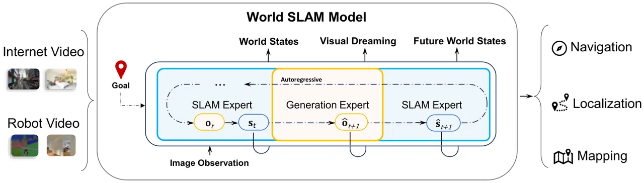
This mixture is more than a concatenation of three networks. Joint attention lets appearance tokens consult metric context and lets geometric tokens exploit texture, occlusion, and motion cues. At the same time, the depth and pose branches need not inherit the full width of a video generator. Separating the parameters respects the very different output spaces: a high-dimensional visual latent and a comparatively compact set of metric states.

The navigation goal $\mathbf{p}_{\mathrm{goal}}$ is a 3D position expressed in the first camera frame, without an orientation. It is encoded as a goal token that conditions only the generation expert through cross-attention. The separation is deliberate. The SLAM expert should estimate what the world is doing, while the generation expert uses the goal to select which future is worth dreaming. Injecting the goal directly into geometric estimation would make it easier for the metric state to explain the desired route rather than measure the actual one.

The goal-conditioned dream is therefore:

$$ \hat{\mathbf{o}}_{t+1}\sim p_\theta\left(\cdot\mid\mathbf{o}_{\leq t},\mathbf{s}_{\leq t},\mathbf{p}_{\mathrm{goal}}\right) $$

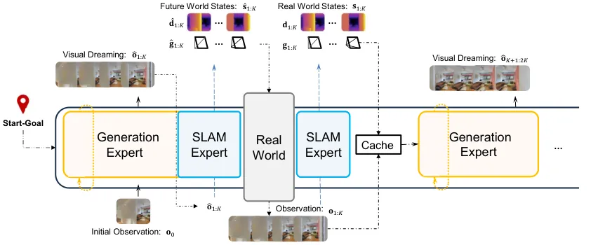
The generated RGB sequence does not become a plan by itself. It must pass back through the SLAM expert, which infers future depth and camera motion. The resulting pose sequence becomes the metric plan followed by the controller. WSM thus inserts an explicit geometry interpretation between the visual dream and the short trajectory prefix that is executed.

Teacher-forced joint pretraining

Each training chunk contains two kinds of tokens. Clean observation tokens $\mathbf{O}_n$ and clean state tokens $\mathbf{S}_n$ provide context. Prediction tokens consist of noisy RGB latents $\mathbf{O}_n^\tau$ and fixed state queries $\bar{\mathbf{S}}_n$, initialized with zero depth and identity pose. An attention mask permits joint supervision of RGB, depth, and pose within the chunk while preserving earlier chunks as causal history. Multiple chunks from an episode can be optimized in one forward pass instead of waiting for a frame-by-frame rollout.

RGB training uses flow matching. With data latent $\mathbf{O}_n$, noise $\boldsymbol{\epsilon}$, flow time $\tau$, and condition $\mathbf{c}_n$, the network $v_\theta$ learns a velocity field from noise toward data:

$$ \mathcal{L}_{\mathrm{FM}}=\mathbb{E}\left[\left\|v_\theta\left(\mathbf{O}_n^\tau,\tau\mid\mathbf{c}_n\right)-\left(\boldsymbol{\epsilon}-\mathbf{O}_n\right)\right\|_2^2\right] $$

Depth is normalized in log space to cover the task's wide metric range:

$$ u=\frac{\log\left(d/d_{\min}\right)}{\log\left(d_{\max}/d_{\min}\right)},\quad d_{\min}=0.2,\ d_{\max}=5 $$

Camera supervision combines absolute and relative pose losses. The first anchors each camera in a common coordinate frame. The second constrains pairwise rigid transforms and therefore emphasizes the local shape of a trajectory:

$$ \mathcal{L}_{\mathrm{abs}}=\sum_j\left\|\hat{\mathbf{g}}_j-\mathbf{g}_j\right\|_\delta,\quad \mathcal{L}_{\mathrm{rel}}=\sum_{i,j}\left\|\hat{\mathbf{g}}_i^{-1}\hat{\mathbf{g}}_j-\mathbf{g}_i^{-1}\mathbf{g}_j\right\|_\delta $$

The complete pretraining objective is a weighted sum of generation, depth, and pose terms:

$$ \mathcal{L}_{\mathrm{pre}}=\mathcal{L}_{\mathrm{FM}}+\lambda_d\mathcal{L}_d+\lambda_p\left(\mathcal{L}_{\mathrm{abs}}+\mathcal{L}_{\mathrm{rel}}\right) $$

This joint objective encourages the video latent space to carry metric structure, but it also exposes a tradeoff. Depth shares the Wan2.2 VAE latent representation, which was designed for appearance generation rather than geometric precision. The convenience of adapting a strong pre-trained video backbone can therefore cost fine surfaces and boundaries, a cost that becomes visible in the reconstruction benchmark.

Closed-loop inference: plan briefly, then return to reality

At each planning step, WSM generates four future RGB latent frames. The SLAM expert converts them into 16 future poses. A low-level controller executes only the first four poses, receives four new RGB observations, updates the history, and replans. This short execution prefix keeps the policy close to real evidence rather than committing to an increasingly speculative generated sequence.

The local backend re-estimates all states that have become available in the current chunk. RGB tokens remain in the KV cache, but their old depth and pose estimates are replaced. Generated frames are not appended to persistent history. The cache therefore contains only real observations and their corrected metric states, preserving a clean distinction between what the robot has seen and what it has merely imagined.

flowchart TD
  A["Observed RGB history"] --> B["SLAM expert estimates depth and pose"]
  B --> C["Persistent observed-state KV cache"]
  C --> D["Generation expert dreams goal-conditioned RGB"]
  D --> E["Same SLAM expert serves as inverse dynamics"]
  E --> F["16 future poses from 4 latent frames"]
  F --> G["Controller executes first four poses"]
  G --> H["Four new RGB observations"]
  H --> B
  H --> I["Local backend re-estimates current chunk"]
  I --> C
  

The uncompressed history cache is both a strength and a liability. It gives the model direct access to accumulated observations, but memory and attention work grow with the number of stored latent frames. In evaluation the cache is capped at 128 observed latent frames. The paper does not report the quality curve beyond that horizon or the latency cost of a full cache, so long-duration navigation remains an open operational question.

Post-training: optimizing the futures that get planned

Pretraining teaches a model to generate plausible continuations and estimate geometry. It does not directly optimize whether a dreamed trajectory is collision-free or makes useful progress toward the goal. The authors therefore post-train on roughly 10 percent of the training trajectories, selected as hard examples. For each query, they sample 16 dreams, use the frozen SLAM expert to recover trajectories, and score them through collision, goal progress, and similarity to an expert route.

The normalized sampling weight is:

$$ r_i=\frac{s_i\exp\left(-C_i/T\right)}{\sum_{j=1}^{G}s_j\exp\left(-C_j/T\right)} $$

Here $s_i$ indicates a collision-free trajectory. The cost $C_i$ compares per-step geodesic progress toward the goal with progress along the expert trajectory. The reward measures whether the robot approaches the goal at an appropriate pace, not whether it reproduces the expert path point by point. A different but safe route can therefore receive a high score. This is important for navigation, where obstacles and local geometry permit many valid trajectories.

Advantages are clipped to define a precision weight:

$$ \rho_i=\frac12+\frac12\operatorname{clip}\left(A_i/A_{\max},-1,1\right) $$

The post-training objective pulls a positive velocity model toward the noise-to-data direction, pushes a negative model away from it, and regularizes the updated model against a reference:

$$ \mathcal{L}_{\mathrm{post}}=\mathbb{E}\left[\rho_i\left\|v^+-\left(\boldsymbol{\epsilon}-\hat{\mathbf{O}}^{(i)}\right)\right\|_2^2+\left(1-\rho_i\right)\left\|v^-\left(\boldsymbol{\epsilon}-\hat{\mathbf{O}}^{(i)}\right)\right\|_2^2\right]+\lambda_{\mathrm{ref}}\left\|v_\theta-v^{\mathrm{ref}}\right\|_2^2 $$

Only self-attention LoRA adapters in the generation expert are updated. The SLAM expert is frozen. This isolates the optimization: the reward cannot be improved by changing the trajectory estimator to reinterpret the same dream more favorably. Any gain can be attributed primarily to a changed distribution of imagined futures. The ablation reports that post-training raises success rate by 5.7 points on Home and 5.4 on Commercial, with SPL gains of 4.8 and 4.9 points.

Navigation benchmark

WSM is trained on InternVLN-N1. Five percent of trajectories are withheld as a SLAM test split and excluded from both pretraining and post-training. Navigation uses the InternVLA-N1 closed-loop start-goal protocol: 40 InternScenes environments, split evenly between Home and Commercial, with 100 episodes per environment. An episode succeeds when the robot slows or stops within one meter of the goal. Results are reported as success rate and success weighted by path length.

All experts are initialized from Wan2.2-5B. The generation expert retains a hidden width of 3072, while depth and pose are initialized with interpolated weights at widths 1536 and 768. Pretraining uses 48 A100 GPUs for 10 epochs, global batch size 48, and random chunk lengths from one to four latent frames. Inference uses one RTX 4090 GPU, 320 by 192 input resolution, four latent frames per plan, eight sampling steps, and 16 predicted poses per plan.

Method	Home SR	Home SPL	Commercial SR	Commercial SPL
DD-PPO	0.4	0.4	5.3	5.2
iPlanner	43.0	40.6	54.6	52.8
ViPlanner	45.0	43.2	63.7	61.9
LoGoPlanner	57.3	52.4	67.1	63.9
LoGoPlanner, re-evaluated	59.6	53.6	65.8	62.0
WSM, RGB only	70.3	66.3	73.9	71.8

WSM is best on both metrics in both environment groups. Relative to the re-evaluated LoGoPlanner, it gains 10.7 success points on Home and 8.1 on Commercial. Relative to LoGoPlanner's published values, the differences are 13.0 and 6.8 points. The smaller gain in Commercial scenes suggests that clutter, reflective surfaces, and less regular layouts remain difficult even with a persistent metric state.

The table also changes how the result should be interpreted. WSM receives only RGB and estimates both camera motion and depth internally. Its advantage is therefore not caused by an extra depth sensor or an external odometry service. The Home SPL of 66.3 is only 4.0 points below its success rate, so successful routes are generally not dominated by severe detours. The main improvement is that more episodes reach the goal at all.

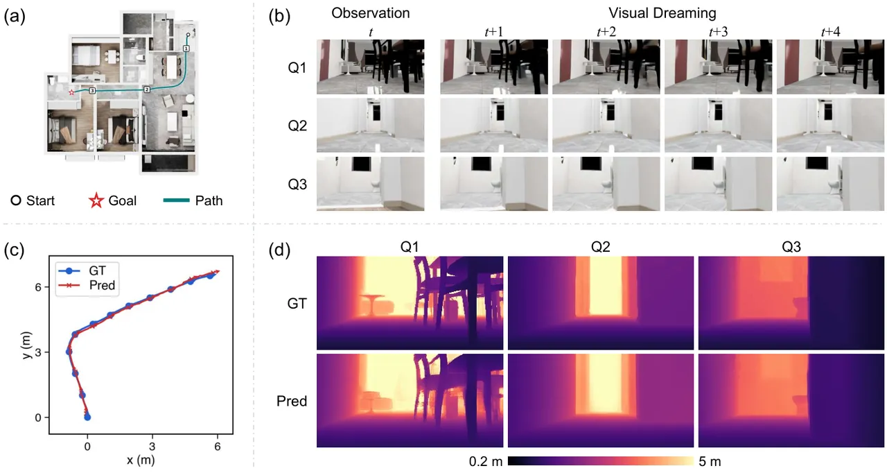
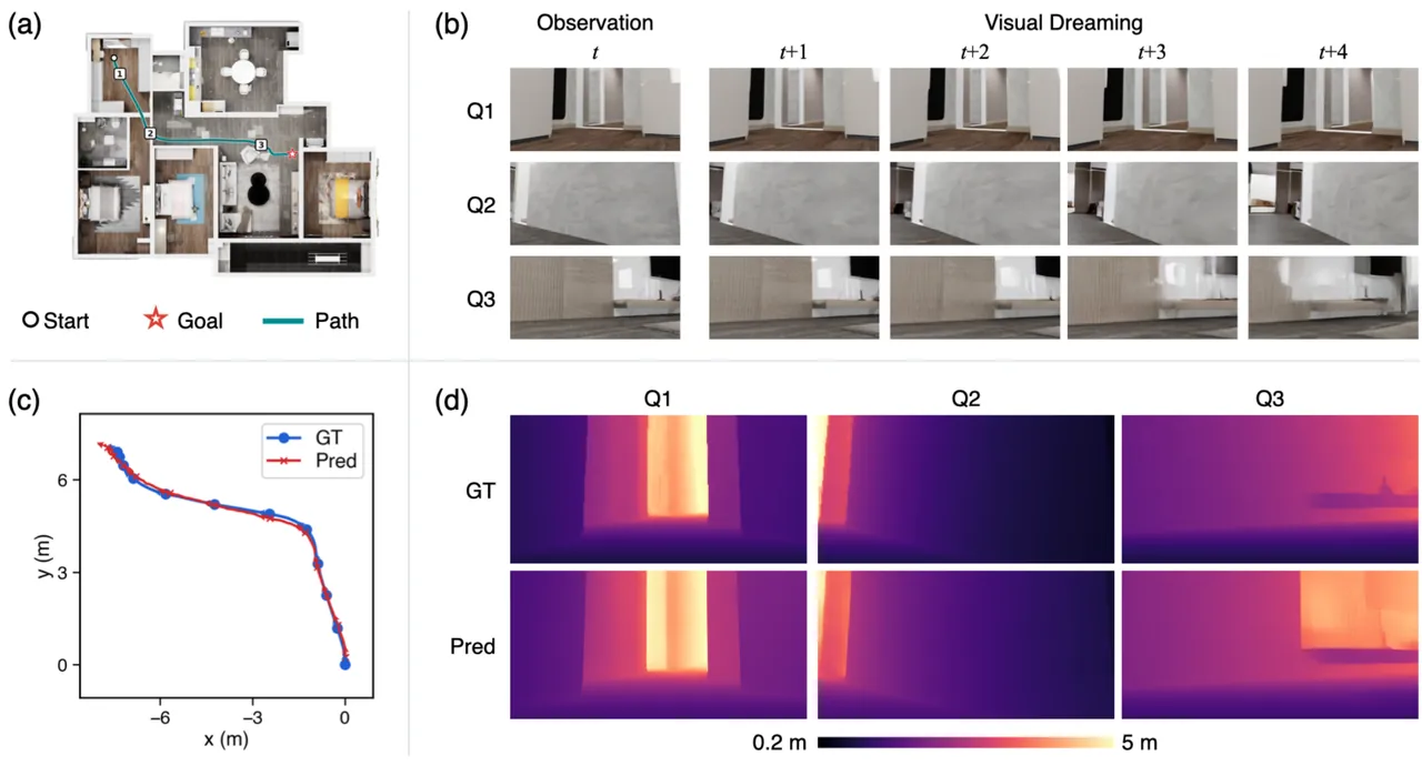
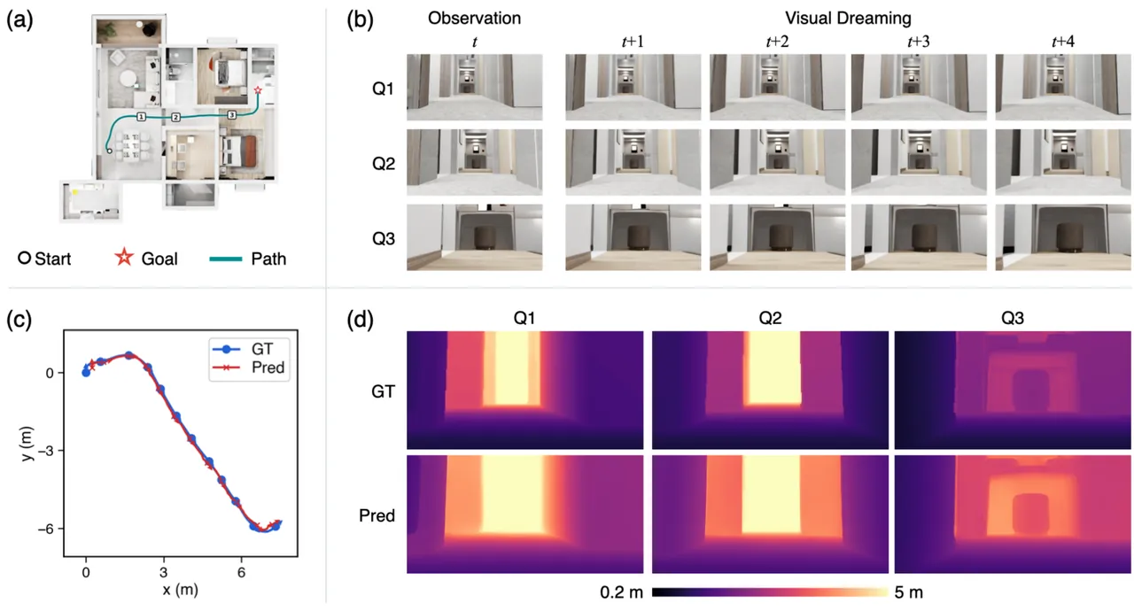
Figure 4 supplies a concrete example of the mechanism working together. The route reaches the goal, the dreamed frames show coherent turns and approach, and the estimated trajectory stays close to the ground truth. The predicted depth follows walls, floor, and furniture boundaries. The authors attribute this agreement to the shared SLAM expert operating on observed and dreamed sequences. The image is still a selected success case, not a distribution of failures, confidence intervals, or uncertainty estimates.

SLAM evaluation: strong pose, weaker dense geometry

SLAM is measured on the reserved 5 percent of InternVLN-N1 trajectories. Camera-center ATE is computed after per-sequence Sim(3) alignment. Dense reconstruction uses the RMSE from predicted points to their nearest ground-truth points after alignment and rigid ICP refinement. WSM is evaluated at 320 by 192, while SLAM-Former uses 518 by 518. WSM is trained on the navigation dataset; SLAM-Former starts from large-scale 3D pretraining and is then fine-tuned on the same navigation training split.

Method	ATE RMSE (m)	Accuracy RMSE (m)
SLAM-Former released checkpoint	0.051	0.057
SLAM-Former fine-tuned	0.041	0.041
WSM	0.021	0.062

The pose result is strong. WSM reaches 0.021 meters ATE, roughly half the 0.041 of fine-tuned SLAM-Former and substantially below its released checkpoint at 0.051. This matters because navigation could otherwise succeed through visually smooth trajectories that have little metric meaning. Here the same model that generates futures also estimates camera positions with substantially lower error on the held-out trajectories.

Dense reconstruction does not show the same advantage. WSM reports 0.062 meters accuracy RMSE, worse than fine-tuned SLAM-Former at 0.041. The authors connect this gap to the appearance-oriented Wan2.2 VAE latent space used for depth, which can soften geometric detail. The result supports a narrow conclusion: WSM is accurate enough for its navigation loop, but it is not a replacement for a dedicated high-fidelity reconstruction system.

The comparison also has limits. Only one SLAM baseline is reported, and its pretrained 3D prior differs from WSM's video-generation initialization. The lower-resolution WSM input could hurt reconstruction, while its stronger pose result may benefit from the navigation objective. A larger benchmark with classical visual SLAM, additional streaming reconstruction models, and matched training data would be needed before making a general SLAM ranking.

Ablations: the mechanism matters

The first ablation compares WSM with an inverse-dynamics-only model. IDM keeps the generation branch and a pose inverse-dynamics branch, but removes depth estimation and the localization of observed frames. It infers motion only from imagined frames. Both models share initialization, training data, and evaluation conditions and are compared before post-training, isolating the effect of maintaining a metric world rather than merely generating transitions.

Method	Home SR	Home SPL	Commercial SR	Commercial SPL
IDM, without SLAM	28.1	27.1	32.1	31.2
WSM, without post-training	64.6	61.5	68.5	66.9

The roughly 36-point success gap is the paper's most consequential ablation. When the goal is fixed in the initial camera frame, a sequence of locally plausible inverse-dynamics estimates is not enough to preserve the global anchor. WSM localizes real frames, maps their geometry, and interprets dreamed frames in the same coordinate system. The plan therefore remains tied to the same goal instead of drifting with the generated video.

The second ablation isolates the local backend. One variant estimates every state once and freezes it. The other jointly re-estimates recent frames within a chunk. Both start from the same pretrained model, are post-trained under their respective update rules, and are evaluated with those same rules.

Method	Home SR	Home SPL	Commercial SR	Commercial SPL
Without backend	68.3	65.2	72.6	70.5
With backend	70.3	66.3	73.9	71.8

The local backend adds 2.0 SR and 1.1 SPL on Home, plus 1.3 SR and 1.3 SPL on Commercial. The effect is modest but consistent in both environment groups. Because the RGB cache is unchanged and only depth and pose estimates are revised, the gain is evidence that correcting states already committed to history reduces accumulated error. It is a useful middle ground between pure incremental estimation and full global optimization.

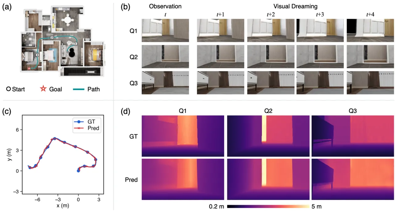
Additional qualitative examples cover four episodes in two Home scenes. Each figure combines a map, selected RGB dreams, estimated and ground-truth trajectories, and predicted depth. These examples make the closed-loop structure easier to inspect, but they do not replace an error breakdown by room type, failure category, collision event, or trajectory length. The paper reports aggregate success and path efficiency rather than a full operational taxonomy.

Limitations and deployment risks

The authors explicitly acknowledge that depth is represented in a Wan2.2 VAE latent space designed for appearance. Geometry therefore trades some fidelity for compatibility with the pretrained video generator. The dense reconstruction result makes the cost concrete: WSM reports 0.062 meters accuracy RMSE against 0.041 for fine-tuned SLAM-Former. Navigation may tolerate this level of geometric softness, but manipulation, thin obstacles, and detailed surface inspection may not.

The authors also acknowledge that the history KV cache is uncompressed. Memory and computation grow with the number of observed frames, which limits long-horizon deployment. The implementation caps inference at 128 observed latent frames, but the paper does not show what happens beyond that budget or how performance changes as the cache fills. A large building, a long inspection route, or a multi-hour task could expose memory and context-retention problems that short episodes do not.

An independent concern is external validity. All reported results come from simulation and offline held-out trajectories. There is no physical robot deployment, so motion blur, changing illumination, wheel slip, dynamic people, calibration error, and actuator delay remain untested. The paper states that inference fits on one RTX 4090, but does not report per-step latency, peak memory, throughput, energy, or achieved control frequency. Hardware feasibility is not the same as real-time deployability.

The baseline coverage is also narrow. Navigation compares four named alternatives, and SLAM compares only SLAM-Former's released checkpoint and a fine-tuned variant. The evaluation does not include a classical visual SLAM system or several recent streaming reconstruction models. Differences in pretraining data and input resolution further limit clean attribution. Stronger claims about state of the art would require matched budgets and a broader set of baselines.

Finally, the public repository is documentation-only at the time of this review. The README says code and checkpoints are coming soon, so the architectural description, equations, and numerical tables can be checked against the paper, but the actual attention masks, local-backend update, reward computation, and training configuration cannot. Reproducibility remains pending until those artifacts are released.

Conclusion

WSM's contribution is not the addition of another generator to a navigation stack. It changes what counts as the world state inside the model. The generation expert proposes possible futures, but the SLAM expert interprets those futures in the same metric coordinates as observed history. Real observations are appended, recent states are refined, and only a short pose prefix is executed before the system returns to new evidence. Generation proposes; metric state constrains; the controller acts briefly and checks again.

The reported evidence supports that joint mechanism. With RGB-only input, WSM reaches 70.3 and 73.9 success on Home and Commercial scenes. Removing SLAM drops the no-post-training comparison to 28.1 and 32.1. Local state refinement and generation-only post-training both add smaller but consistent gains. At the same time, WSM's worse dense reconstruction score and missing physical deployment data define the boundary of the claim.

The most important next step is geometry-native latent state. If depth were represented for geometry rather than appearance, reconstruction fidelity might improve without giving up the shared video backbone. Compressed or hierarchical history could also control long-horizon memory, while real-robot testing would expose latency, motion, and recovery failures that simulation hides. Until then, WSM is a strong architectural argument with promising benchmark evidence, not yet a deployable general SLAM replacement.

Golden quote: A useful world model must do more than imagine a plausible future. It must keep that future accountable to one spatial reality that every new observation can correct.