PAPER DEEP DIVE
LeWAM: End-to-End World and Action Modeling with JEPAs
Joint-embedding predictive architectures (JEPAs) learn compact latent world models without pixel reconstruction. Existing JEPA pipelines typically train visual representations and action-conditioned dynamics before adding a control policy or solver. We introduce LeWAM, an end-to-end JEPA for control with: (1) a joint training objective over next latent state prediction and action flow matching, and (2) an isotropic Gaussian constraint on the latent state, enabling a single model to support direct policy execution and efficient planning by evaluating sampled actions with its learned latent dynamics. Compared with prior JEPAs in visual planning, LeWAM improves success rate from 28.6% to 89.7% on contact-rich tasks and from 10.9% to 46.2% on long-horizon tasks, and plans 32.3 times faster. On behavior cloning tasks in simulation and physical robots, LeWAM is also competitive with established methods. Interpretability analyses show that LeWAM learns control-relevant representations and action distributions effectively guiding test-time planning and control.
Paper Information
Title: LeWAM: End-to-End World and Action Modeling with JEPAs.
Source: arXiv:2610.12818. The full paper is available at https://arxiv.org/abs/2610.12818 , the project page at https://le-wam.github.io/ , and the official code at https://github.com/MinghaoFu/lewam .
Code status: The repository contains the encoder, Mixture-of-Transformers predictor, training objective, gradient planner, CEM, and behavior-cloning evaluation. The released training config sets the frame skip to 5, the SIGReg weight to 0.04, and the action-flow inference to 8 Euler steps, matching the paper's description.
One-Sentence Summary
LeWAM jointly learns action-conditioned latent dynamics, an action flow-matching policy, and visual representations in one end-to-end model. It can execute action chunks directly or freeze its network and refine candidate action sequences through its latent world model. Across ten visual-planning environments, it reaches an average success rate of 93.5%, 42.7 percentage points above LeWM with CEM; on four long-horizon tasks with a 100-step goal offset, it reaches 46.2% versus 10.9% for the baseline. It also plans at 52.50 plans per second, 32.3 times faster.
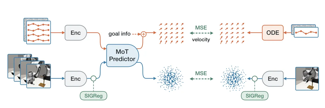
Figure 1: LeWAM training overview (paper Figure 1). The same encoder encodes history, goal, and future observations. Clean actions supervise latent-state prediction; noisy actions supervise flow-matching action learning.
Motivation
Visual control requires more than a map from pixels to actions. A useful policy must anticipate how candidate actions change object poses, contacts, and robot state. World models address this by letting a controller imagine outcomes before executing them. Joint-embedding predictive architectures are attractive for this role because they predict future states in a compact latent space instead of reconstructing pixels.
Existing JEPA pipelines often separate representation learning, action-conditioned dynamics, and policy learning. One common recipe freezes a pretrained visual encoder and trains dynamics or inverse dynamics on top of it. Another trains a world model first and attaches an action predictor afterward. These designs simplify engineering, but they disconnect action supervision from visual representation learning. If the latent space drops control-relevant detail, planning becomes brittle; if it retains irrelevant detail, search becomes expensive.
The planning side has its own tension. CEM initialized from a broad Gaussian prior needs many candidates and rollouts to discover feasible behavior. The problem worsens as action dimensionality increases, horizons lengthen, or contact modes switch. A separately trained action predictor can provide a better prior, but when it is trained on frozen features, action information cannot shape the encoder.
LeWAM answers by putting the three components in one training stage. A shared encoder learns observation representations. A Mixture-of-Transformers predictor simultaneously predicts future latent states and action velocities. SIGReg constrains the latent distribution and prevents collapse. At inference, the action branch is both a direct policy and a source of planning candidates; the state branch both imagines consequences and scores candidates against a goal.
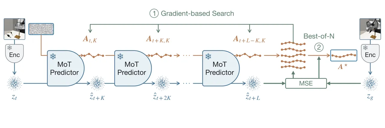
Figure 2: Position of LeWAM (paper Figure 2). Unlike frozen-encoder pipelines, external solvers, or world-model-then-policy recipes, it constrains representation, dynamics, and action distribution within one training objective.
Problem Formulation
Let $\boldsymbol{o}_{1:T}$ denote observations, $\boldsymbol{a}_{1:T}$ actions, and $\boldsymbol{z}_t=\mathrm{Enc}(\boldsymbol{o}_t)$ the latent of frame $t$. Time indices are raw environment steps. The frame skip $K$ means that one state-dynamics prediction advances 5 environment steps; the policy chunk length $C$ means that one action-flow sample contains 10 contiguous actions. The history contains two recent latents, and goal-conditioned tasks add a goal-image embedding plus a normalized remaining horizon.
The two predictor branches are:
$$\hat{\boldsymbol{z}}_{t+K}=f_z(\boldsymbol{q}_{t+K}^z;\boldsymbol{z}_{\leq t},\boldsymbol{A}_{t,K}),\qquad \hat{\boldsymbol{v}}_{t,C}=f_a(\boldsymbol{A}_{t,C}^{(s)};s,\boldsymbol{z}_{\leq t},\boldsymbol{c}_t).\tag{1}$$
Here $\boldsymbol{A}_{t,C}^{(s)}$ is the noisy action chunk at flow time $s$, and $\boldsymbol{q}_{t+K}^z$ is a learned state query. Integrating the action branch's velocity field yields an action chunk. The branches share attention but keep modality-specific query, key, value, and feed-forward projections.
Architecture
The simulation visual-planning encoder uses a ResNet-18-style convolutional backbone. Convolutional layers use GroupNorm with 16 groups. Inputs are randomly cropped from $224\times224$ to $202\times202$ during training and center-cropped at evaluation. A $1\times1$ convolution produces 32 spatial maps. Spatial softmax pooling converts each map into the expectation of normalized image coordinates, giving 64 features. A two-layer MLP with BatchNorm then projects 64 features through 384 hidden units to a 192-dimensional latent.
The Mixture-of-Transformers predictor has width 192, 4 blocks, 4 attention heads, and dropout 0.1. Its token sequence contains two history latents, one learned state query, five clean action tokens, and ten noisy action-flow slots. Learned type and positional embeddings distinguish these groups. The visual-planning model has about 16.9M trainable parameters, deliberately small enough for per-task training and fast test-time search.
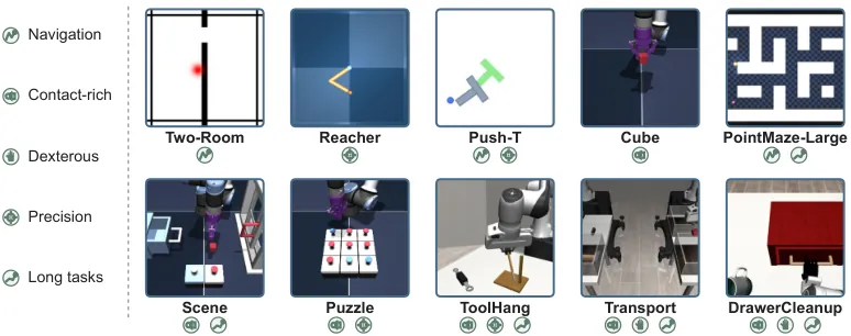
Figure 3: The MoT attention mask (paper Figure 3). Filled cells permit attention and white cells are masked, preventing clean actions or state targets from leaking into the action-flow branch through history latents.
Without the optional goal context, the token sequence is:
$$[\boldsymbol{z}_{t-\Delta},\boldsymbol{z}_t,\boldsymbol{q}_{t+K}^z,\boldsymbol{A}_{t,K},\boldsymbol{A}_{t,C}^{(s)}].\tag{2}$$
The clean action group expands into five tokens and the noisy action group into ten tokens. The state query reads both history latents and clean actions. Each noisy action token reads history and its own causal prefix. History tokens attend only to history and never read actions. This isolation prevents the action branch from indirectly seeing clean target actions through attention.
Training Objective
Flow matching interpolates a recorded action chunk with Gaussian noise and regresses the velocity from noise toward data. For $s\in[0,1]$ and $\boldsymbol{\epsilon}\sim\mathcal{N}(\boldsymbol{0},\boldsymbol{I})$:
$$\boldsymbol{A}_{t,C}^{(s)}=(1-s)\boldsymbol{\epsilon}+s\boldsymbol{A}_{t,C},\qquad \boldsymbol{v}_{t,C}=\frac{\mathrm{d}\boldsymbol{A}_{t,C}^{(s)}}{\mathrm{d}s}=\boldsymbol{A}_{t,C}-\boldsymbol{\epsilon}.\tag{3}$$
The state and action losses are mean squared errors:
$$\mathcal{L}_{\mathrm{dyn}}=\mathbb{E}_{\mathcal{D}}\!\left[\mathrm{MSE}(\hat{\boldsymbol{z}}_{t+K},\boldsymbol{z}_{t+K})\right],\qquad \mathcal{L}_{\mathrm{act}}=\mathbb{E}_{\mathcal{D},s,\boldsymbol{\epsilon}}\!\left[\mathrm{MSE}(\hat{\boldsymbol{v}}_{t,C},\boldsymbol{A}_{t,C}-\boldsymbol{\epsilon})\right].\tag{4}$$
SIGReg imposes an isotropic Gaussian distributional constraint to prevent JEPA collapse. Let $\boldsymbol{Z}$ collect history and target latents in a minibatch, $\boldsymbol{u}^{(m)}$ be random unit directions, and $T$ be the Epps–Pulley test statistic against a standard normal distribution:
$$\mathcal{L}_{\mathrm{sig}}=\frac{1}{M}\sum_{m=1}^{M}T(\boldsymbol{Z}\boldsymbol{u}^{(m)}).\tag{5}$$
The full objective combines the three terms with $\lambda_{\mathrm{sig}}=0.04$:
$$\mathcal{L}_{\mathrm{LeWAM}}=\mathcal{L}_{\mathrm{dyn}}+\mathcal{L}_{\mathrm{act}}+\lambda_{\mathrm{sig}}\mathcal{L}_{\mathrm{sig}}.\tag{6}$$
Goal conditioning enters only the noisy action tokens. It contains a goal-image embedding and a normalized remaining horizon. The horizon is converted into a 128-dimensional sinusoidal embedding and modulates noisy action slots through AdaLN-Zero blocks with hidden width 512. Without a goal, the same model reduces to goal-free behavior cloning; with a goal, it supports visual goal reaching.
Direct Execution and Gradient Planning
For direct execution, LeWAM integrates the learned velocity field from Gaussian noise. The paper uses 8 Euler steps:
$$\frac{\mathrm{d}\boldsymbol{A}_{t,C}^{(s)}}{\mathrm{d}s}=f_a(\boldsymbol{A}_{t,C}^{(s)};s,\boldsymbol{z}_{\leq t},\boldsymbol{c}_t),\qquad \boldsymbol{A}_{t,C}^{(0)}\sim\mathcal{N}(\boldsymbol{0},\boldsymbol{I}),\qquad \hat{\boldsymbol{A}}_{t,C}=\boldsymbol{A}_{t,C}^{(1)}.\tag{7}$$
During planning, the model first samples $N$ candidates from its action distribution. At each imagined stage, the first 5 actions of each candidate advance its latent dynamics, the predicted latent is appended to a fixed-length history, and the remaining goal horizon is updated. After building the full candidate, the model is frozen and only the normalized action plan is optimized through the latent goal cost:
$$\mathcal{C}(\boldsymbol{A})=\mathrm{MSE}(\hat{\boldsymbol{z}}_{t+L}(\boldsymbol{A}),\boldsymbol{z}_g).\tag{8}$$
Action $k$ is updated as:
$$\boldsymbol{a}_{t+k}\leftarrow\boldsymbol{a}_{t+k}-\eta\frac{\partial\mathcal{C}}{\partial\boldsymbol{a}_{t+k}},\qquad k=0,\ldots,L-1.\tag{9}$$
The implementation adds a quadratic proximity penalty to keep refinement near the sampled proposal. With $\boldsymbol{A}^{\mathrm{sample}}$ denoting the candidate before refinement:
$$\mathcal{J}_{\mathrm{prox}}(\boldsymbol{A};\boldsymbol{A}^{\mathrm{sample}})=\mathcal{C}(\boldsymbol{A})+\lambda_{\mathrm{prox}}\left\|\boldsymbol{A}-\boldsymbol{A}^{\mathrm{sample}}\right\|_F^2.\tag{10}$$
Candidate retention and final selection use the unpenalized goal cost. Adam uses learning rate 0.05, gradient-norm clipping 10, normalized action clipping $a_{\max}=3$, and $\lambda_{\mathrm{prox}}=0.01$. The planner executes the first 5 actions, observes the environment, and repeats sampling, imagination, refinement, and execution. On Push-T, success plateaus after 5 Adam updates; more updates increase latency without a consistent gain. Increasing candidates beyond 8 also gives no consistent gain in the reported sweep.

Figure 4: LeWAM planning (paper Figure 4). Each stage samples candidate action chunks, advances imagined states with the first five actions, refines complete candidates by gradient descent, and executes the best plan.
flowchart TD
    O["Current observation"] --> E["Shared encoder"]
    E --> H["Latent history"]
    H --> M["Mixture-of-Transformers"]
    M --> Z["State branch
predicts z_t+5"]
    M --> A["Action branch
predicts 10-step action flow"]
    A --> S["Sample 32 candidates"]
    S --> R["Frozen network
latent rollout"]
    R --> C["Latent goal MSE"]
    C --> G["5 Adam refinements
proximity penalty, action clipping"]
    G --> B["Select lowest-cost candidate"]
    B --> X["Execute first 5 actions"]
    X --> O
Evaluation Protocol
Visual planning gives the model a goal image and asks it to reach the depicted state from a random starting state within a fixed action budget. Task completion gives no goal image and evaluates behavior cloning from start to finish. The ten simulated environments span navigation and manipulation, with different action dimensions, camera views, data provenance, and trajectory lengths. Four environments follow LeWM's setup; six add mazes, interacting objects, coupled buttons, precise tool placement, bimanual transport, and drawer cleanup. For Cube, success checks both object and end-effector positions to avoid false positives from an object-only predicate.
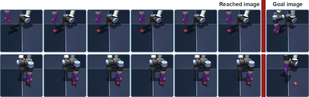
Figure 5: Ten simulation environments (paper Figure 5). The suite covers 2-D manipulation, 3-D object manipulation, maze navigation, and bimanual coordination under a single architecture.
Visual Planning Results
With a 25-step goal offset and a 50-action budget, LeWAM exceeds LeWM plus CEM on all ten tasks, averaging 93.5% success versus 50.9%. The largest gap appears on the contact-rich bimanual Transport task, where LeWAM scores 83.3% and LeWM only 2.8%. ToolHang improves from 35.4% to 94.7%. On the logically structured Puzzle task, LeWAM reaches 80.7% while goal-conditioned GCBC reaches 44.0%.
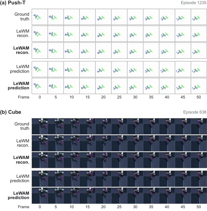
Figure 6: Visual planning results (paper Figure 6). Most tasks use a 25-step goal offset and 50-action budget; Two-Room follows LeWM's 100-step goal offset and 150-action budget, and LeWM uses 10 seeds for stability.
The long-horizon sweep moves goals to recorded frames 25, 50, 75, or 100 steps later while keeping the start fixed at the first frame. Across Push-T, Cube, Scene, and Puzzle, LeWAM averages 46.2% success at a 100-step offset, while LeWM averages 10.9%. The learned action prior therefore does not merely shorten short-horizon search; it also keeps behavior candidates meaningful over longer sequences.
| Task | Method | 25 steps | 50 steps | 75 steps | 100 steps |
|---|---|---|---|---|---|
| Push-T | LeWAM | 94.7 ± 3.1 | 60.7 ± 3.1 | 44.0 ± 3.5 | 43.3 ± 4.6 |
| Push-T | LeWM | 68.7 ± 3.1 | 12.0 ± 4.0 | 3.3 ± 2.3 | 2.7 ± 1.2 |
| Cube | LeWAM | 100.0 ± 0.0 | 88.0 ± 2.0 | 80.7 ± 2.3 | 82.0 ± 2.0 |
| Cube | LeWM | 100.0 ± 0.0 | 0.0 ± 0.0 | 4.0 ± 3.5 | 4.0 ± 3.5 |
| Scene | LeWAM | 82.7 ± 3.1 | 73.3 ± 8.1 | 65.3 ± 3.1 | 56.0 ± 4.0 |
| Scene | LeWM | 44.7 ± 13.0 | 31.3 ± 2.3 | 37.3 ± 5.8 | 36.0 ± 6.0 |
| Puzzle | LeWAM | 74.0 ± 12.5 | 14.0 ± 3.5 | 4.0 ± 3.5 | 3.3 ± 1.2 |
| Puzzle | LeWM | 10.0 ± 0.0 | 4.7 ± 2.3 | 4.0 ± 2.0 | 0.7 ± 1.2 |
Table 1: Goal-reaching success by horizon, in percent (paper Table 5). Puzzle remains difficult at 100 steps, but LeWAM improves both absolute success and relative margin.
Planning speed is central. LeWM uses $300\times30$ CEM; LeWAM uses 32 sampled candidates and 5 Adam refinements. Across Scene, Puzzle, Cube, and Push-T, LeWAM averages 52.50 plans per second versus 1.62 for LeWM, a 32.3 times speedup. The gain comes from a low-entropy action prior and batched gradient refinement on a GPU.
| Task | Action dim. | LeWM ms/plan | LeWM plans/s | LeWAM ms/plan | LeWAM plans/s | Speedup |
|---|---|---|---|---|---|---|
| Scene | 5 | 705 | 1.42 | 18.8 | 53.19 | 37.5× |
| Puzzle | 5 | 731 | 1.37 | 16.3 | 61.35 | 44.8× |
| Cube | 5 | 771 | 1.30 | 21.1 | 47.39 | 36.5× |
| Push-T | 2 | 414 | 2.42 | 20.8 | 48.08 | 19.9× |
| Mean | — | — | 1.62 | — | 52.50 | 32.3× |
Table 2: Planning speed (paper Table 6). All neural networks are timed on the same H100. One plan is one full planner call, not one model forward pass.
Representations, Dynamics, and Action Distributions
Linear probes show that joint action supervision improves decodable control information. Compared with LeWM, LeWAM raises average proprioception, action, and inverse-dynamics $R^2$ by 0.21, 0.20, and 0.19. SIGReg is also more than an anti-collapse trick: on Push-T, removing it reduces the planning gain from 14.7 to 2.7 percentage points. Removing SIGReg from LeWM drives object, proprioception, and action probes to $R^2=0$.
| Environment | Model | SIGReg | Effective rank | Object $R^2$ | Proprio $R^2$ | Action or IDM $R^2$ |
|---|---|---|---|---|---|---|
| Push-T | LeWAM | Yes | 42.90 | 0.90 | 0.86 | 0.40 (0.75) |
| Push-T | LeWAM | No | 10.94 | 0.88 | 0.85 | 0.38 (0.73) |
| Push-T | LeWAM MSE head | No | 6.96 | 0.66 | 0.86 | 0.36 (0.74) |
| Push-T | LeWM | Yes | 94.20 | 0.95 | 0.80 | 0.29 (0.71) |
| Push-T | LeWM | No | 16.23 | 0.00 | 0.00 | 0.00 (0.00) |
Table 3: Push-T linear probes and effective rank (paper Table 1). Parenthesized inverse-dynamics probes use both current and future latents.
The end-to-end encoder also matters. Averaged over Push-T, Cube, Scene, and Puzzle, LeWAM's jointly trained features score 86.7% for direct control and 91.5% with planning. Frozen DINOv2 CLS features score 79.0% and 82.7%; frozen DINOv2 patch-mean features score 75.8% and 77.7%. Joint training therefore changes features in ways that action selection actually needs, rather than merely supplying a generic visual prior.
| Visual encoder | Mode | Push-T | Cube | Scene | Puzzle | Average |
|---|---|---|---|---|---|---|
| LeWAM end-to-end | Direct | 85.3 ± 5.0 | 100.0 ± 0.0 | 88.0 ± 6.9 | 73.3 ± 5.8 | 86.7 |
| LeWAM end-to-end | Planning | 98.7 ± 1.2 | 100.0 ± 0.0 | 93.3 ± 3.1 | 74.0 ± 12.5 | 91.5 |
| Frozen DINOv2 CLS | Direct | 72.7 ± 7.6 | 98.7 ± 1.2 | 82.0 ± 4.0 | 62.7 ± 7.0 | 79.0 |
| Frozen DINOv2 CLS | Planning | 78.7 ± 6.4 | 99.3 ± 1.2 | 91.3 ± 1.2 | 61.3 ± 13.0 | 82.7 |
| Frozen DINOv2 patch mean | Direct | 66.0 ± 12.5 | 93.3 ± 2.3 | 84.0 ± 2.0 | 60.0 ± 7.2 | 75.8 |
| Frozen DINOv2 patch mean | Planning | 67.3 ± 8.1 | 98.7 ± 1.2 | 86.0 ± 4.0 | 58.7 ± 7.6 | 77.7 |
Table 4: Visual-encoder ablation (paper Table 8). Direct mode uses no test-time search; planning mode refines candidates through learned dynamics. Success rates are in percent.
The value of a stochastic action distribution is clearest in a two-door navigation study. The demonstrations use a fixed start and goal, with half passing through an upper door and half through a lower door. The flow-matching action head follows both routes in closed-loop rollouts. Replacing it with a deterministic MSE head collapses behavior toward the lower route and produces some wall collisions. Flow matching therefore preserves a conditional action distribution, not merely a conditional mean.
To test whether the action branch harms dynamics learning, the authors remove the action head at evaluation and plan with CEM using only the state branch. LeWAM scores 84.0% on Push-T, slightly below LeWM's 92.4%, but 86.0% on Cube, 22.2 points above LeWM's 63.8%. Together with open-loop visual rollouts, this shows that action supervision and state prediction can reinforce rather than compete with each other.
Behavior Cloning and Real Robots
Goal-free behavior cloning retains state prediction and action flow matching but removes goal conditioning. On simulated task completion across DrawerCleanup, Transport, and ToolHang, LeWAM averages 64.7% versus 61.6% for Diffusion Policy. Transport improves from 45.3% to 61.3%; Diffusion Policy remains stronger on ToolHang, 84.7% versus 80.0%.
The real-robot suite covers Pick and Place T, Push-T, and Tape Stack with 30 trials per task. End-to-end LeWAM averages 33.3%; the frozen V-JEPA 2.1 encoder variant averages 35.6%; Diffusion Policy averages 38.9%; and π0.5 averages 28.9%. End-to-end LeWAM does not surpass Diffusion Policy in average success, but it is much cheaper at inference: one full action-chunk inference costs 270.2 GFLOPs, versus 3603.6 GFLOPs for π0.5, a 13.3 times difference in operation-count efficiency.
| Method | Pick and Place T | Push-T | Tape Stack | Average | GFLOPs |
|---|---|---|---|---|---|
| Diffusion Policy | 19/30 | 16/30 | 0/30 | 38.9% | 270.0 |
| π0.5 | 14/30 | 3/30 | 9/30 | 28.9% | 3603.6 |
| LeWAM frozen encoder | 15/30 | 12/30 | 5/30 | 35.6% | 270.2 |
| LeWAM end-to-end | 16/30 | 8/30 | 6/30 | 33.3% | 270.2 |
Table 5: Real-robot results over 30 trials (paper Table 2). GFLOPs counts one full action-chunk inference, including all denoising or Euler integration steps.
The data scale frames the claims. The simulation suite totals about 71,988 trajectories, 13.1M frames, and 235.5 hours, combining expert demonstrations, random-policy interactions, and mixed-quality data. Models are trained or adapted separately per task and embodiment rather than trained once across all tasks. The paper does not claim a universal multi-task robot foundation model; its focus is whether a 16.9M model can support both direct policy execution and test-time planning.
Code and Implementation Details
In the official code, `lewam/models/encoders.py` implements the GroupNorm ResNet encoder, spatial softmax, and BatchNorm projector; `lewam/models/lewam.py` implements MoT blocks, token layout, flow loss, and ODE integration; `lewam/eval/planners.py` implements gradient planning, best-of-k, steering, and CEM; `scripts/train_lewam.py` combines state, action, and SIGReg losses; and `configs/train/base.yaml` fixes frame skip 5, action chunk 10, SIGReg weight 0.04, and 8 flow steps. These details map directly to the equations above.
There are two training recipes. Goal-conditioned visual planning uses batch size 128, 50 epochs, base learning rate $1.5\times10^{-4}$, and 5 warmup epochs. Goal-free task completion uses batch size 64, 120 epochs, base learning rate $10^{-4}$, and 10 warmup epochs. Both use AdamW, weight decay $10^{-4}$, cosine learning-rate decay, gradient-norm clipping 1, and seed 42. The data split is 90/10, and checkpoints are selected by lowest validation action-flow loss, not by task success.
Limitations and Failure Modes
First, data coverage remains limited. The suite combines expert and non-expert data but does not cover the full range of contact transitions, unstructured scenes, or exploratory behavior. The authors note that broader play data would likely help contact-rich tasks.
Second, generalization is not fully tested. Most evaluations remain within similar visual distributions and task-internal goal construction. Unfamiliar objects, viewpoints, and contact states require further study.
Third, models are trained or adapted separately per task and embodiment. This is not yet a multi-task, multi-embodiment, or language-conditioned policy. Shared dynamics can only scale after broader data and multi-task training.
Fourth, planning remains low-level continuous control. Longer tasks that require subgoal decomposition, symbolic constraints, or task-stage switching still need a hierarchical planner.
Fifth, both training and test-time search are small. The visual-planning model has about 17M parameters, uses 32 candidates, and applies 5 Adam refinements. Larger models may learn more general dynamics but will change the latency tradeoff.
Sixth, contact handling remains heuristic. The appendix explicitly says that rigorous guarantees for 3-D contact-rich manipulation are future work. The proximity penalty, action clipping, and flow prior are practical choices rather than complete contact-mode reasoning.
One experimental boundary deserves emphasis: LeWAM's real-robot average success is lower than Diffusion Policy's. The work reduces π0.5's 3603.6 GFLOPs to 270.2 GFLOPs and demonstrates efficiency, but Table 2 should not be read as overall superiority on physical manipulation.
Conclusion
LeWAM's contribution is to connect a policy prior and world-model imagination through the same gradients. The action flow is not an isolated imitation head; it gives test-time search a low-entropy starting distribution. Latent-state prediction is not dynamics that only work in offline evaluation; it is shaped by action supervision and retains control-relevant detail. Direct execution handles fast reactions, while planning corrects deviations, and both share one 16.9M-parameter model.
For robot-system designers, the key lesson is that priors can matter more than candidate count. CEM needs 9,000 candidates from a broad prior; LeWAM uses 32 candidates and 5 refinement steps to achieve higher success. That difference makes a latent world model closer to real-time control than to a research-only slower planner. The 32.3 times acceleration on contact-rich tasks also shows that a learned action distribution is itself an optimizable search structure.
Even so, LeWAM is not the full answer for general robot foundation models. Per-task training, limited data, lower real-robot average success than Diffusion Policy, and the absence of hierarchical planning all bound its scope. It is a strong and clean end-to-end JEPA control proof, not a finished system for every robot problem.
Key Takeaways
The action distribution is both policy and search prior. When candidates come from a learned flow model, test-time optimization starts near feasible behavior instead of blind noise.
A latent world model must retain control-relevant detail. Joint state, action, and distributional constraints shape the encoder so that goal-cost gradients point toward actions that change physical outcomes.
References
Paper: https://arxiv.org/abs/2610.12818
Project: https://le-wam.github.io/
Code: https://github.com/MinghaoFu/lewam