RSI-Anything: Unlocking Recursive Self-Improvement with World Models

Paper: RSI-Anything: Unlocking Recursive Self-Improvement with World Models (arXiv:2610.13912, arxiv.org/abs/2610.13912, v1 submitted 2026-10-09, primary class cs.CL)
Authors: Taoyong Cui, Pinxian Zeng, Wanghan Xu, Hao Xiao, Shuhan Xue, Qiang Gao, Wanli Ouyang, Pheng Ann Heng, Zhenfei Yin, Yingcheng Wu, Ling Yang (PhAI Labs, CUHK, University of Macau, SJTU, Fudan, Oxford, Stanford, Peking University; corresponding authors Pheng Ann Heng, Zhenfei Yin, Yingcheng Wu, Ling Yang)
Code status: public. Gen-Verse/RSI-Anything (Apache-2.0, 298 stars, last push 2026-10-12, 707 files) with model and data assets under Hugging Face Gen-Verse/RSI-Anything. Reproducibility is tiered: code repair and GUI interaction ship complete runnable workflows (rsi run --config configs/code_repair/default.json), while laboratory planning and reaction optimization ship inference-side adapters plus sealed evaluation records, and the immune-science application is documentation only. Every claim below about the implementation was read off the main branch.

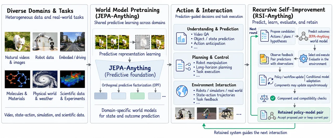
Figure 1: RSI-Anything at a glance (paper Figure 1). JEPA-Anything supplies cross-domain prediction; those predictions support understanding, planning and action selection. Interaction feedback drives policy or workflow updates and conditionally triggers world-model adaptation, and component plus compatibility checks decide which policy-model pair is retained to steer the next round of interaction and learning.

In One Sentence

RSI-Anything treats recursive self-improvement as a version-control problem: a world model prices each candidate before any expensive feedback is spent, feedback then proposes changes to two separately versioned components, and a pair of acceptance gates decides which combination survives into the next cycle, so that improvement accumulates instead of evaporating. With the coder frozen, hidden-test success on code repair climbs from 26.3% for a static verifier to 29.2% with predictive selection and 31.2% after world-model adaptation; over five retained policy versions, LabHorizon F200 goes from 21.80% to 46.01%.

Background: The Expensive Part Is Feedback, Not Parameters

Recursive self-improvement means turning interaction experience into durable gains in both what a system can do and how it learns. The paper separates two timescales that the literature routinely blurs. Within a task, feedback repairs the current solution or steers the next action; verifiers and Reflexion-style reflection live here. Across cycles, self-training and preference optimization convert experience into persistent policy or workflow revisions. The word "recursive" only earns its keep on the second timescale, because an update that is not retained cannot change what happens next. The research question is therefore stated plainly: how does the experience from one round improve the system's ability to act and to learn in the round after it.

The first obstacle is price. Learning from external feedback requires executing or measuring a candidate before its consequences exist, and when the interaction budget is capped, that price directly shrinks the exploration space. In code repair one purchase is a sandboxed test round; in chemistry it is a real bench operation; in immunology it is a wet-lab experiment. This is where a world model earns its slot: by predicting the consequences of candidate actions on subsequent states or outcomes, it makes thinking-before-doing possible, and it lets scarce feedback be spent on the candidate that is most informative or most promising. The authors frame the world model as the predictive foundation for improvement under limited external feedback.

The substrate is the group's own prior work, JEPA-Anything. It follows the joint-embedding predictive route, predicting target representations from an observation context rather than reconstructing pixels, and adds orthogonal prediction decomposition: the latent target is split into complementary factors, each factor gets a dedicated predictor, and factor outputs are recombined into a complete latent state. That decomposition is what lets one modelling skeleton serve heterogeneous domains such as images, control and molecular dynamics. The authors are explicit about where the prior work stops: prediction is not recursive improvement. A predicted outcome has to steer interaction, and external feedback has to produce updates that survive across cycles. Neither responsibility belongs to JEPA-Anything.

Wiring those two responsibilities together runs into what the paper calls coupled updates, and this is the sharpest problem statement in the document. Change the policy and the distribution of candidate actions and of experience changes with it, yet the world model was trained and evaluated on the old distribution, so its predictive reliability may no longer hold. Change the world model and candidate ranking, imagined trajectories, and the learning signal fed to policy improvement all change. The conclusion is uncomfortable: improving either component in isolation does not guarantee that the assembled system is better. Reliable recursion therefore needs three things that most self-improvement papers skip, namely a rule for deciding when to update which component, an evaluation of predictive reliability conditional on a changed policy, and a guarantee that the retained policy-model pair actually improves subsequent interaction and learning.

RSI-Anything answers by promoting retention to a first-class operation. Policy and world model are allowed to evolve asynchronously: component-level checks judge each update on its own, a compatibility check judges the assembled pair, and only a version that clears both enters the next cycle. Three contributions follow. First, a predictive world model is wired into RSI and the unit of persistent improvement is lifted from a single policy to a policy-world-model system, which makes predictive reliability under an evolving policy a design requirement rather than a post-hoc audit. Second, an update-and-retention protocol chains prediction-guided selection, feedback-driven improvement, conditional model adaptation, and component plus pair acceptance. Third, the protocol is exercised across code repair, GUI interaction, laboratory planning and reaction optimization, with an end-to-end immune-science application on top.

Preliminaries: What a Run May Change and What It Must Not

Each domain $d$ is described by an eight-part task specification:

$$\mathcal{T}_{d}=\left(\mathcal{X}_{d},\ \mathcal{S}_{d},\ \mathcal{A}_{d},\ \mathcal{W}_{d},\ \mathcal{V}_{d},\ \mathcal{M}_{d},\ \mathcal{C}_{d},\ \mathcal{B}_{d}\right). \tag{1}$$

Here $\mathcal{X}_{d}$ covers observations and context, $\mathcal{S}_{d}$ the task state, $\mathcal{A}_{d}$ the admissible actions or interventions, $\mathcal{W}_{d}$ the world-model adapter, and $\mathcal{V}_{d}$ the verifier responsible for candidate validity and predictive utility; the remaining three entries are the evaluation metrics, the runtime and safety constraints, and the budget for computation, simulation and external interaction. The adapter deserves a remark of its own, because it is what makes attribution possible later: it binds each piece of external feedback to the stored prediction it was compared against, to the action and context that produced that prediction, and to the evidence source. Every reliability statement downstream depends on that binding existing.

Two independent clocks are used. $t$ indexes actions inside a task; $k$ indexes update-and-acceptance cycles. The system accepted in cycle $k$ is the pair $(\theta_{k},\phi_{d,k})$, where $\theta_{k}$ is the policy configuration, which may be trainable parameters or a persistent agent workflow, and $\phi_{d,k}$ is the current predictor. One cycle can aggregate many action steps, trajectories or even tasks, and it ends once the update decision and the acceptance checks are complete, including the case where both components keep their previous versions. So $k$ counts update cycles, not successful revisions, a distinction that matters when reading the five policy versions in the laboratory experiments.

Table 1 of the paper sorts the objects in a run into four classes with explicit change rules. It looks like formal scaffolding, but it is actually the gate that stops a longer memory from being sold as self-improvement: only accepted changes to $\theta$ or $\phi_{d}$ count as system revisions.

Object	Change rule	What carries into the next cycle
Task and evaluation specification	Fixed for the whole run	Objectives and definitions, interfaces, evaluation criteria, constraints, budget caps, acceptance and stopping rules
Task state and experience	Actions and observations rewrite the state and append prediction-observation records to history	The state seen by later actions; the accumulated record used for selection and learning
Policy configuration $\theta$	Feedback-driven policy learning or workflow rewriting proposes a candidate version; the component gate and the pair gate decide acceptance	The accepted policy configuration, otherwise the current one is carried over
World model $\phi_{d}$	An adaptation attempt is triggered only when prediction is unreliable, data is sufficient and budget allows; the same two gates apply	The accepted predictor, otherwise the current one is carried over

Table 1: fixed quantities, update rules and retained state within one recursive run (paper Table 1). The in-run budget only decreases; task state, candidate pool, feedback records and accepted component versions may evolve.

The predictive substrate: encode, predict, read out

JEPA-Anything supplies the context-to-target predictive design, orthogonal prediction decomposition organizes the latent target, and its training objective mixes factor prediction with orthogonality and representation regularization. RSI-Anything inherits this substrate, but the adaptation stage is allowed to declare its own objective and its own trainable parameter subset. Encoding and action-conditioned latent prediction in cycle $k$ are written

$$z_{t}=E_{\phi_{d,k}}\left(s_{t},c_{d}\right), \tag{2}$$

$$\widehat{z}_{t+1}=F_{\phi_{d,k}}\left(z_{t},a_{t},c_{d}\right), \tag{3}$$

with $s_{t}$ the task state, $a_{t}$ the candidate action and $c_{d}$ the domain context. Where orthogonal prediction decomposition is instantiated, $F$ denotes the two steps of factor prediction followed by factor composition. A readout $R$ turns the predicted latent target into outcome predictions usable for selection and for comparison against feedback, and the paper stresses that these symbols name functional roles: action encoding is up to the adapter and may be folded into the predictor input or into the context.

$$\widehat{o}_{t+1}=R_{\phi_{d,k}}\left(\widehat{z}_{t+1},c_{d}\right)\quad\text{(point readout)}, \tag{4}$$

$$p_{\phi_{d,k}}\left(o_{t+1}\mid s_{t},a_{t},c_{d}\right)=R_{\phi_{d,k}}\left(\widehat{z}_{t+1},c_{d}\right)\quad\text{(probabilistic readout)}. \tag{5}$$

A point readout is assessed with outcome error; a probabilistic readout can additionally be scored with distribution-sensitive or calibration metrics. Any uncertainty estimator used for selection or for training admission must be declared separately. That requirement reappears in the reliability section, and it is the paper's consistent style: every quantity that can move a decision gets a name and a provenance.

Single-step selection needs only the outcome readout. Multi-step planning additionally needs an adapter that can advance the planning state, and where that transition interface exists the rollout under goal $g$ and horizon $H$ is

$$p_{\theta_{k},\phi_{d,k}}\left(\widehat{\tau}\mid s_{0},g,c_{d}\right)=\prod_{t=0}^{H-1}\pi_{\theta_{k}}\left(a_{t}\mid s_{t},g\right)\,p_{\phi_{d,k}}\left(s_{t+1},o_{t+1}\mid s_{t},a_{t},c_{d}\right). \tag{6}$$

The paper attaches a qualifier that is easy to skim past: until it is externally validated, the propagated $s_{t+1}$ is only a predicted planning state. A joint transition readout is required by rollout applications alone, which is why code repair, a single-step selection task, never needs one.

Method: Six Steps, Two of Which Are Gates

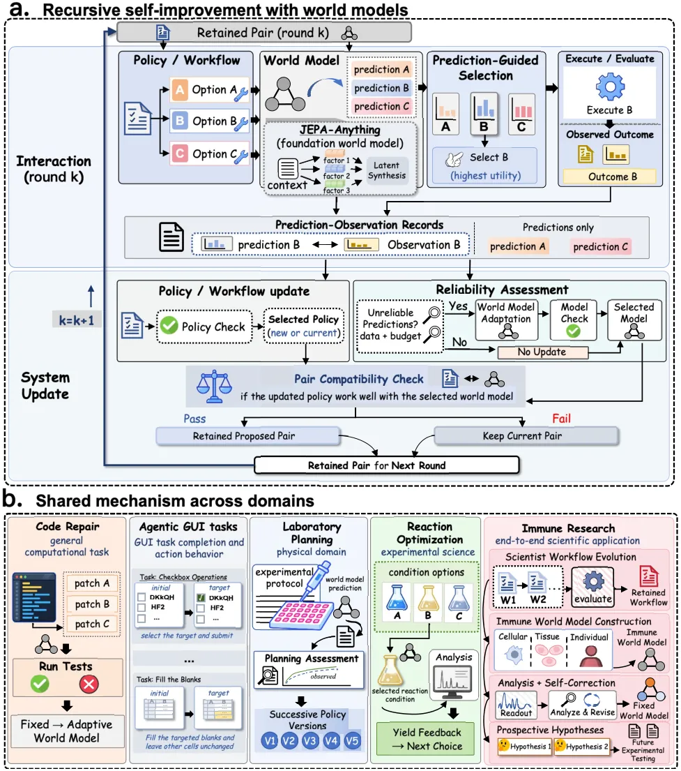
Figure 2: the framework (paper Figure 2). Panel a: on top of JEPA-Anything, world-model predictions guide candidate selection and only the executed candidate B produces external feedback. Panel b: the same mechanism instantiated for code repair, GUI interaction, laboratory planning and reaction optimization, with immune science chaining the retained workflow and predictor into an end-to-end application.

Steps one to three: propose, predict, select on utility

Given state $s_{t}$ and goal $g$, the current policy proposes a candidate set $\mathcal{K}_{t}=\operatorname{Propose}_{\theta_{k}}\left(s_{t},g\right)$. Each candidate receives an outcome prediction, or a bounded rollout $\widehat{\tau}$ where the transition interface supports one. The verifier then records validity $v_{\tau}$, utility components $\mathbf{r}_{\tau}$, evidence provenance, and whatever model or verifier uncertainty is available. There is a deliberate split of labour here: validity and runtime constraints decide which candidates are allowed to run at all, while the selection rule decides which feasible candidates actually go and buy feedback. Utility-based ranking scores

$$R_{d}\left(\widehat{\tau}\right)=\sum_{j}w_{d,j}\,r_{\tau,j}-\Delta_{d}\left(\widehat{\tau}\right), \tag{7}$$

where $\Delta_{d}\left(\widehat{\tau}\right)=\lambda_{d}\,U\left(\mathbf{u}_{\tau}\right)$ when an uncertainty penalty is enabled and $\Delta_{d}\left(\widehat{\tau}\right)=0$ otherwise. Invalid candidates are removed before ranking. The domain configuration owns the utility weights, the ranking or acquisition rule actually in force, the batch size and the estimated cost of feedback; selection returns one feasible candidate or a batch whose evaluation cost fits inside the remaining feedback budget. In code repair the instantiated rule aggregates predicted execution-class probabilities, ranks the four proposed revisions, and executes exactly one of them.

The paper leaves a second branch open: if an information-seeking acquisition rule is explicitly enabled, the system prefers to evaluate uncertain candidates instead. Its definition and its usage must be reported separately from utility ranking, because the two optimize different objectives and reporting them together would make the claim that prediction helps impossible to interpret. Once feedback arrives, the observation and the prediction that was used to select that candidate are stored separately, which is what keeps the reliability estimate honest later.

Evidence tiers and the admission of imagined data

Evidence comes in four tiers: deterministic rule checks (E0), learned-model predictions and rollouts (E1), specialized simulators or higher-fidelity calculations (E2), and external measurements or experiments (E3). Predicted fields and observed fields keep their own provenance. The tier records origin and intended fidelity; whether a record is good enough to train on is decided by a separate admission criterion, and that separation is the point.

$$e_{\tau}=\mathbf{1}\left\{v_{\tau}=1\right\}\ \mathbf{1}\left\{R_{d}\left(\widehat{\tau}\right)\geq r_{d}^{\min}\right\}\ C_{d}^{U}\left(\widehat{\tau}\right)\ \mathbf{1}\left\{\ell_{\tau}\in\mathcal{E}_{d}^{\mathrm{train}}\right\},$$

$$\mathcal{D}_{\mathrm{sim},k}=\operatorname{Curate}\left\{\widehat{\tau}:e_{\tau}=1\right\}. \tag{8}$$

$\ell_{\tau}$ records the evidence supporting this training admission. The uncertainty check $C_{d}^{U}$ tests $U\left(\mathbf{u}_{\tau}\right)\leq u_{d}^{\max}$ when enabled and returns 1 otherwise, with allowed evidence sources and thresholds declared per application. If imagined learning is disabled, $\mathcal{D}_{\mathrm{sim},k}$ is empty. The authors add one sentence that carries a lot of weight: this training filter does not prevent the system from externally evaluating an uncertain candidate. Refusing to train on a record and refusing to spend an experiment on it are different decisions, and the second one may be exactly where the money should go.

Steps four and five: two improvement paths off the same feedback

External feedback appends prediction-observation pairs to the history $\mathcal{H}_{k}$, each bound to the system version that produced it. Records selected for policy improvement form $\mathcal{D}_{\mathrm{policy},k}$; records selected for predictor adaptation form $\mathcal{D}_{\mathrm{adapt},k}$. The two sets serve different objectives and need not contain the same records. Policy improvement changes how candidates are generated or chosen; predictor adaptation changes how their consequences are forecast.

Feedback must first be converted into a signal that matches the thing being updated: imitation treats the selected action or trajectory as a target, preference learning compares candidates using evaluation outcomes, and workflow search ranks persistent agent workflow configurations by evaluation feedback. Each application picks the path implied by its policy representation, and eligible imagined trajectories may supplement policy data when that route is enabled. Writing $u_{k}^{\pi}$ for a policy update attempt at a declared schedule or feedback trigger, with the required learning evidence and sufficient budget, a fixed-policy setting is simply $u_{k}^{\pi}=0$:

$$\theta^{\prime}_{k+1}=\begin{cases}\operatorname{Update}\left(\theta_{k},\mathcal{D}_{\mathrm{policy},k},\mathcal{D}_{\mathrm{sim},k}\right),&u_{k}^{\pi}=1,\\ \theta_{k},&u_{k}^{\pi}=0.\end{cases} \tag{9}$$

An instantiated route has to state three things: how feedback constructs training targets or workflow scores, which parameters or configuration fields may change, and when an update is attempted. The headline code-repair experiment deliberately pins $u_{k}^{\pi}$ to zero so that any observed gain can only come from selection and from the predictor; laboratory planning does the opposite and follows the policy version sequence alone. Reading the two experiments together is what separates the contributions.

Conditional world-model adaptation: reliability must be attributable to the current version

Adaptation uses observed targets to improve the corresponding prediction. One constraint is easy to miss: outcome labels can supervise the outcome readout, but latent prediction targets require an observation that the domain target encoder can represent. A scalar outcome supplies an outcome target, not a full observed target state, even though its loss can propagate into upstream trainable parameters. An adaptation declaration therefore states the available targets, its predictive loss and the trainable parameter subset, and these choices may differ from the initial modelling stage.

The reliability protocol requires predictions to be attributable to the current model version: for each historical observation included in the assessment, either use the prediction that this version generated and stored, or re-apply the current model to the recorded inputs to obtain a fresh prediction. Predictions from earlier versions remain usable for analysing past decisions but must not be mixed into the current error estimate. With $\mathcal{K}_{k}$ the candidate range considered in cycle $k$, $B_{\mathrm{update},k}$ the remaining budget and $\widehat{c}_{\mathrm{adapt},k}$ the estimated cost in the same units, assessment and trigger read

$$\rho_{k}^{W}=\operatorname{Reliability}\left(W_{\phi_{d,k}};\mathcal{H}_{k},\mathcal{K}_{k}\right)\in\left\{\mathrm{reliable},\ \mathrm{unreliable},\ \mathrm{insufficient}\right\}, \tag{10}$$

$$u_{k}^{W}=\mathbf{1}\left\{\rho_{k}^{W}=\mathrm{unreliable}\right\}\ \mathbf{1}\left\{\mathcal{D}_{\mathrm{adapt},k}\ \mathrm{is\ sufficient}\right\}\ \mathbf{1}\left\{B_{\mathrm{update},k}\geq\widehat{c}_{\mathrm{adapt},k}\right\}, \tag{11}$$

$$\phi^{\prime}_{d,k+1}=\begin{cases}\operatorname{Adapt}\left(\phi_{d,k},\mathcal{D}_{\mathrm{adapt},k}\right),&u_{k}^{W}=1,\\ \phi_{d,k},&u_{k}^{W}=0.\end{cases} \tag{12}$$

The insufficient state is the load-bearing one. Because feedback only arrives for selected candidates, any conclusion holds only over the observed and covered candidate range, so thin coverage must be reported as insufficient evidence rather than as apparent reliability, and it must not fire the adaptation trigger. That single design choice writes selection bias into the protocol instead of hoping it away. The trigger additionally requires sufficient data and sufficient budget simultaneously, and a disabled path has $u_{k}^{W}=0$ identically. Budget declarations must name the constrained resource and count adaptation, history re-evaluation and acceptance checks; where policy and model share a budget, each attempt uses the balance left after earlier allocations. External feedback usage and update or evaluation compute are reported separately.

Step six: recursive retention, and why a pair gate is not redundant

The retention protocol compares the proposed components and the pair they assemble against the current versions under pre-declared acceptance criteria. Component checks cover two things: policy task utility and constraints, or predictor quality on the relevant targets. The pair check covers the dependency between them, because a policy can generate candidates on which an otherwise improved predictor is unreliable, and a predictor changes which candidates get selected. Pair acceptance therefore concerns the decision behaviour of the assembled system and predictor suitability on the candidates the selected policy actually proposes, which is beyond the isolated quality of either part. Formally, with the comparison baseline written into the parameter list:

$$G_{k}^{\pi}=Q_{\pi}\left(\theta^{\prime}_{k+1};\ \theta_{k},\ \mathcal{D}^{\pi}_{\mathrm{gate},k}\right), \tag{13}$$

$$G_{k}^{W}=Q_{W}\left(\phi^{\prime}_{d,k+1};\ \phi_{d,k},\ \mathcal{D}^{W}_{\mathrm{gate},k}\right), \tag{14}$$

where each check returns 1 only if its declared criteria are met. The versions entering pair evaluation are

$$\bar{\theta}_{k+1}=\begin{cases}\theta^{\prime}_{k+1},&u_{k}^{\pi}=1\ \wedge\ G_{k}^{\pi}=1,\\ \theta_{k},&\text{otherwise},\end{cases}\qquad \bar{\phi}_{d,k+1}=\begin{cases}\phi^{\prime}_{d,k+1},&u_{k}^{W}=1\ \wedge\ G_{k}^{W}=1,\\ \phi_{d,k},&\text{otherwise}.\end{cases} \tag{15,16}$$

If at least one component changed, the pair decision compares the assembled candidate pair with the current pair under the same prescribed evaluation conditions; if neither changed, $G_{k}^{\mathrm{pair}}=1$ and no new evaluation is run:

$$G_{k}^{\mathrm{pair}}=Q_{\mathrm{pair}}\left(\left(\bar{\theta}_{k+1},\bar{\phi}_{d,k+1}\right);\ \left(\theta_{k},\phi_{d,k}\right),\ \mathcal{D}_{\mathrm{compat},k}\right), \tag{17}$$

$$(\theta_{k+1},\phi_{d,k+1})=\begin{cases}\left(\bar{\theta}_{k+1},\bar{\phi}_{d,k+1}\right),&G_{k}^{\mathrm{pair}}=1,\\ \left(\theta_{k},\phi_{d,k}\right),&\text{otherwise}.\end{cases} \tag{18}$$

Failure handling is asymmetric on purpose: a failed component check keeps that component's current version, while a failed pair check rolls the whole pair back. Data is split three ways as well, with update data constructing candidate versions, gate data deciding which version is retained, and a designated held-out audit set used only for final reporting. The evaluation specification fixes task metrics, prediction checks, constraints, feedback allowance and acceptance thresholds, and task conditions can be matched even when two policies generate different candidates. The retained pair then enters the next cycle together with the accumulated feedback history: a changed policy alters which candidates are proposed, a changed predictor alters ranking and learning signals, and jointly they determine which actions receive feedback and what experience later updates get to see. That dependency of subsequent interaction and learning on already-retained revisions is exactly what the paper means by recursion.

flowchart TD
  CAND[Candidate pool K_t proposed by policy theta_k] --> E0[Tier E0 deterministic rule checks]
  E0 -->|invalid| DROP[Rejected before ranking]
  E0 -->|valid| E1[Tier E1 world model prediction and bounded rollout]
  E1 --> UTIL[Utility R_d as weighted sum minus uncertainty penalty]
  UTIL --> BUD[Budget test against remaining feedback credit]
  BUD --> E3[Tier E3 external execution or bench measurement]
  E3 --> HIST[History H_k stores prediction observation pair with version id]
  HIST --> DPOL[D_policy_k feeds policy update candidate]
  HIST --> DADP[D_adapt_k feeds reliability assessment]
  DADP --> REL[Rho_k_W resolves to reliable unreliable or insufficient]
  REL -->|reliable| KEEP[Predictor stays at phi_d_k]
  REL -->|insufficient coverage| KEEP
  REL -->|unreliable and data sufficient and budget allows| ADAPT[Adapt produces candidate predictor]
  DPOL --> GP[Component gate G_k_pi against current policy]
  ADAPT --> GW[Component gate G_k_W against current predictor]
  KEEP --> GW
  GP --> PAIR[Pair gate G_k_pair under matched conditions]
  GW --> PAIR
  PAIR -->|pass| RETAIN[Retained pair becomes cycle k plus 1 start]
  PAIR -->|fail| ROLLBACK[Whole pair reverts to current versions]
  RETAIN --> CAND
  ROLLBACK --> CAND

Figure 3: the loop reconstructed from Sections 2.1 to 2.5 and Equations 7 to 18, organized by evidence tier. The three-valued reliability verdict is what makes the left branch cheap: thin coverage keeps the predictor frozen instead of triggering an adaptation that the data cannot support.

How the five domains bind to the protocol

Table 4 of the paper aligns state, action, world model, prediction target, policy or workflow, and feedback source for each domain, and it annotates the update scope actually reported everywhere. This is the table to keep open while reading the experiments, because it states outright that each experiment instantiates only part of the full protocol.

Domain	State and action	World model and prediction target	Policy or workflow and feedback-driven change	Feedback and evaluation
Code repair	Programs, tests and feedback; candidate revisions	W1 built on JEPA-Anything, adapted from Qwen2.5-Coder-3B-Instruct with LoRA; probabilities over five execution outcome classes	Fixed ReasonFlux-Coder-7B; W1 either frozen or adapted from feedback	Execution test feedback; final test-suite pass rate and online test usage
GUI interaction	Interface state and task; GUI actions	GUI outcome predictor; consequences of candidate interface actions	Both the action policy and the world model are updated from interaction feedback	Task outcomes; completion rate and action-level diagnostics
Laboratory planning	Protocol context; candidate action sequences	JEPA-Anything-based protocol model; predicted consequences of candidate sequences	A 4B planning policy; five consecutive versions from the same self-improvement process	Development feedback; L1 next-action accuracy and L2 Final Score on F200
Chemical reaction	Reactions; condition vectors	ReactionT5-JEPA-Anything; yield distributions	Measured yields steer subsequent condition selection	GC and LC-MS measured yields; best observed yield at matched experiment counts
Immune science	Cellular, tissue and individual context; interventions	Immune world model; multi-scale transitions and biological readouts	Workflow evolution and world-model construction; predictor frozen during downstream analysis	Measured perturbations support modelling; withheld interventions and contexts evaluate predictions

Table 2: domain bindings and the update scope each one reports (paper Table 4). The world model forecasts consequences; the policy proposes or selects actions.

Code Correspondence: Where the Symbols Live

The repository separates a shared workflow from domain tasks. src/rsi_anything/ is a standard-library-only runner exposing plan, run, status and report; domain implementations live under tasks/<domain>/ with their own interpreter and pinned dependencies, and the JEPA core is vendored at vendor/jepa-anything-core. The README compresses the whole framework into six verbs, Propose, Predict, Select, Evaluate, Learn, Retain, matching the six operations in paper Figure 2. Four correspondences below can be checked line by line on main.

One: W1 is tasks/code_repair/src/world.py::ExecutionWorld. The paper describes W1 as a 3B execution-outcome world model using the JEPA-Anything predictive design, adapted from Qwen2.5-Coder-3B-Instruct with LoRA, returning per-candidate probabilities over execution outcome classes. In source that expands as follows. DomainEncoder attaches LoraConfig(r=16, lora_alpha=32, lora_dropout=0.0, target_modules=['q_proj','k_proj','v_proj','o_proj']) to a bfloat16 backbone, mask-mean-pools token outputs into Linear(hidden, 256) + LayerNorm, and caps input length at 16384 tokens, raising Overlength rather than truncating silently. With mode='opf' it composes OrthogonalFactorProjection(D=256, K=4, R=64, learnable=True, orthogonality_mode='soft_gram') and UnconstrainedMultiHeadPredictor, which is precisely the factor-predict-then-compose reading of $F$ in Equation 3. The readout head is LayerNorm(256) -> Linear(256,64) -> GELU -> Linear(64,6): the first five logits are the five execution statuses AC, WA, TLE, RE and CE, and the sixth passes through softplus to predict runtime seconds, i.e. the probabilistic readout of Equation 4 plus a resource channel. The training objective is

loss = representation + ce + 0.1 * resource + 0.2 * ranking
# ce      = cross_entropy(output[:, :5], labels)
# resource= smooth_l1(softplus(output[:, 5]), seconds)
# ranking = mean relu(0.1 - p_good + p_bad)  # same group_id, differing AC status
# representation = jepa_anything_objective(...).total  # prediction + orthogonality
#                                       + factor_activity + encoder_variance

The representation term calls the vendored jepa_anything_objective directly, with an EMA target encoder at decay 0.996 encoded under torch.no_grad(); the stop-gradient implied by Equations 2 and 3 is an explicit .detach() plus an assertion that target parameters carry no gradient. Scoring at inference uses a learnable temperature, softmax(readout(z)[:, :5] / log_temperature.exp().clamp(0.2, 5.0)), and the optimizer splits parameters into three learning-rate groups (LoRA 5e-6, readout head 1e-4, OPF 1e-5, AdamW weight decay 0.01) with the temperature excluded from all of them. Grouping by role and assigning different rates is exactly what the paper means when it says adaptation declares its own trainable subset, possibly different from the initial modelling stage.

Two: Equations 7 and 8 are implemented in semantic_world.py, with leakage assertions attached. That file extends W1 with a whole-training-suite head: suite_readout deep-copies the original readout, swaps the final Linear(64, 6) for Linear(64, 7), copies the first six rows of weights verbatim and zeroes the seventh, so the extension is an existing head plus one new channel rather than a retrained head. The seventh channel passes a sigmoid to predict pass fraction, and utility is hard-coded as

utility = P(full training suite passed) + 0.25 * predicted pass fraction
predicted_utility = softmax(suite[:, :5])[:, 0] + 0.25 * sigmoid(suite[:, 6])

That is Equation 7 instantiated for code repair with $w_{d,1}=1$, $w_{d,2}=0.25$ and no uncertainty penalty. validate_scope() then turns the admission criterion of Equation 8 into runtime assertions: every transition must declare a prediction_scope of either per_public_test or whole_training_suite, aggregate rows must carry the g6-whole-training-suite-transition-v1 schema, observed pass fraction must lie between 0 and 1, status==0, allpass and partial==1 must be mutually consistent, and utility must equal allpass + 0.25 * partial within 1e-8. Finally four provenance flags must all be False: context_contains_private_case_inputs, context_contains_private_expected_outputs, target_contains_candidate_code and gate_or_final_labels_used. In plain terms, no private test inputs or expected outputs may appear in the context, the target may not contain the candidate code itself, and neither gate data nor final evaluation labels may enter training. The paper's sentence about predicted and observed fields retaining their own provenance is four booleans in code. The listwise loss uses a KL divergence against softmax targets at temperature 0.1 and enforces that every pool is a complete set of four distinct candidates from the same execution transition; pools with identical utility are skipped, singletons with only keep_initial are skipped, and the skip counts are reported.

Three: "matched evaluation conditions" is string splitting in incumbent.py::state_signature. The paper says task conditions can be matched even when two policies generate different candidates. The implementation slices each record's context at '\nCandidate action:\n' to recover the prior state and at '\nOfficial public test suite:\n' to recover the suite, asserts both delimiters are present, and returns (before, tests) as the signature. make_units() then asserts that the initial unit has step_id == -1 and candidate_id == 'keep_initial' and is unique in its group, that first-round units have step_id == 0 with exactly four candidates, and that all four candidates share the incumbent's state signature exactly. Those five rows form one comparison unit, four candidates plus one incumbent, which is what Equations 13 to 18 need in order to compare under identical conditions. Units also carry a contrast flag for whether the maximum utility in the group exceeds the minimum; batches_for() fills position zero with contrastive units first, uses four distinct tasks per batch, reuses consumed units when a batch cannot be filled and records their indices in padding_indices, and finally asserts that the multiset of all indices equals Counter(range(len(rows))), i.e. every row is used exactly once.

Four: the external evaluator under E3, with E0 in front of it, is the sandbox in cure_wm.py; its five status codes are the first five readout logits. execute() runs compile() first and records CE for every test on a syntax error or an empty program; each test then runs under runuser -u nobody -- unshare -Urn -- python -I candidate.py, and with sandbox='required' a host missing runuser or unshare raises instead of degrading. Subprocess limits are RLIMIT_CPU=(10,11), RLIMIT_AS=1GiB, RLIMIT_FSIZE=1MiB and RLIMIT_NOFILE=64, with the environment reduced to PATH=/usr/bin:/bin. After the default three-second timeout the whole process group is killed with killpg(SIGKILL) and marked TLE; a non-zero return code is RE; stdout.strip() == expected.strip() is AC, otherwise WA. These five codes align exactly with the five classification logits of the readout head, so W1 is not learning an abstract notion of quality but the five outcomes this sandbox can emit plus a runtime. An empty test suite raises ValueError: no tests, no feedback, as a hard error.

Orchestration. tasks/code_repair/src/training.py splits predictor construction and adaptation into four stages, initial -> semantic -> expanded -> incumbent, each consuming the previous checkpoint, mirroring the documented sequence of verifying assets, updating the initial, semantic, expanded and incumbent worlds, then evaluating. Several assertions are worth naming: assert len(rows) == config['rows'] with verify_training_hash() pins training-set content and hash; assert not train_ids & dev_ids and not train_ids & set(experiment()['evaluation']['tasks']) forces training, development and evaluation tasks to be disjoint; the semantic stage trains heads only via set_update_stage('heads') before joint training, excluding log_temperature from the trainable set in both; after each step update_ema() runs with gradients clipped to norm 1 and error_if_nonfinite=True; and after saving, the checkpoint is reloaded and rescored on the same four contexts with assert torch.allclose(..., rtol=2e-5, atol=2e-6), which blocks silently corrupted checkpoints between stages. Metadata records final200_labels_used=False, matching the paper's rule that the held-out set is for final reporting only. On the GUI side, src/rsi_anything/tasks/gui.py renders the paper's statement that the retained pair is used for subsequent interaction as a fixed stage sequence, prepare-models -> doctor --gpu -> freeze -> preflight browser -> preflight world -> adapt-and-evaluate, emitting protocol.json, base_manifest.json, two *_contracts.json files, outputs/results.json and outputs/completion_audit.json. Freezing the protocol before running means the three controller configurations are compared under one frozen evaluation protocol, and adapt-and-evaluate contains two policy or world updates, one conditional confirmation, an audit and an aggregation.

Experiments

Code repair: freeze the coder, vary only selection and predictor

This is the cleanest comparison in the paper precisely because the policy is pinned. ReasonFlux-Coder-7B proposes four revisions with at most three feedback rounds; all four selection methods share the same coder and the same candidate budget; evaluation covers 200 CodeContests problems across three random seeds, giving 600 problem-seed evaluations, with online tests supplying feedback during selection and hidden tests supplying the final success measure. The results only mean something when read next to usage: replacing random selection with world-model-guided selection moves hidden-test full-pass rate from 26.0% to 29.2% (175 of 600), and letting the predictor adapt on execution feedback moves it to 31.2%, while online test-suite calls stay at 3.71 to 3.72 across all four methods.

Selection method	Hidden-test full pass rate	Online test calls per task
Random-K, pick one candidate at random	26.0%	3.72
Capacity-matched static verifier	26.3%	3.72
RSI-Anything with fixed world model (CURE-WM-Lite)	29.2%	3.71
RSI-Anything with world-model adaptation	31.2%	3.72

Table 3: three-round repair under a shared coder and candidate budget (paper Table 2; 200 CodeContests problems times three seeds, 600 evaluations). Both RSI-Anything configurations use world-model-guided candidate selection and differ only in whether the world model is updated from feedback.

Two prediction-quality metrics explain where the gain comes from. Candidate-ranking accuracy rises from 66.5% for the static verifier to 72.8%, and the five-class Brier score falls from 0.488 to 0.358. Better ranking means the same four execution chances are more likely to be spent on a good candidate; a lower Brier score means the probabilities themselves are usable, which matters because the utility in Equation 7 is a weighted sum of probabilities, and an uncalibrated probability makes the ranking rule degenerate. The paired gain over the static verifier is +2.83 percentage points with a 95% interval of [+0.17, +5.50]. Note that this number is not the difference of the two rounded rates (29.2 minus 26.3 is 2.9), because it is computed per problem-seed pair with tasks as the cluster-resampling unit. The lower bound of +0.17 means this gain just clears zero statistically, and it should not be inflated when quoted. Separately, on APPS Introductory (1000 problems, 3000 problem-seed evaluations) and LiveCodeBench v6 (1055 problems, 3165 evaluations), JEPA-Anything-guided candidate selection reaches final full-test success of 46.37% and 33.05%, above random selection and the static verifier, reported as arithmetic means over three seeds. All methods share the initial program per problem and seed, repair is guided by public tests, repair stops when all public tests pass, and final success requires passing the complete official suite.

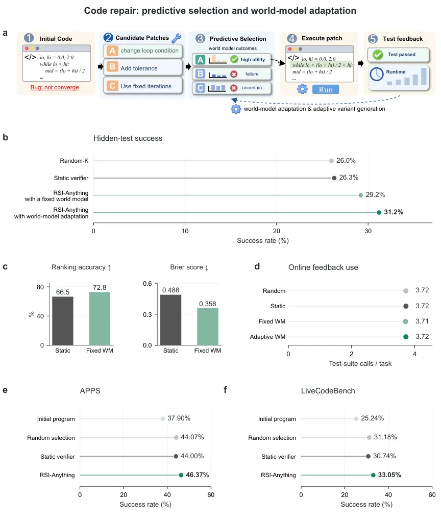
Figure 4: code repair (paper Figure 3). Panel a shows repairing a non-converging loop, from candidate patches and predicted outcomes to execution and test feedback, with A to C as example patches; the benchmark itself uses a fixed coder and four candidates per round. Panels b to d report results on 200 CodeContests problems over three seeds with at most three feedback rounds: b final hidden-test full-pass rate, c candidate-ranking accuracy and five-class Brier score, d mean online test calls per task. Panels e and f give final full-test success over three seeds on APPS Introductory and LiveCodeBench v6. Green is the world-model method, gray the baselines.

GUI: success rate and action economy have to be read together

The MiniWoB++ click-checkboxes task requires checking the boxes named by an instruction and submitting the form. Evaluation uses the same 100 test instances with a per-episode cap of 120 seconds and eight actions, and success requires every checkbox state to match the instruction with the form submitted. RSI-Anything updates both the action policy and the world model from interaction feedback, and the retained pair is used for subsequent interaction. Success across the three retained configurations is 51%, then 79%, then 99%, against 49%, 96% and 98% for the World-based control.

Metric	Initial	Adapted configuration	Final configuration
Task success rate	51%	79%	99%
Mean actions per episode	5.30	2.93	3.21
Episodes with incorrect submissions	9	21	1
Recorded repeated clicks	237	not reported	0

Table 4: behaviour of the three retained configurations on click-checkboxes (paper Figure 4c and 4e to 4g, plus repository docs/benchmarks.md). Actions per episode fall 39.4% from baseline, 5.30 to 3.21.

The middle configuration is the one worth stopping on. It uses the fewest actions at 2.93 and reaches 79% success, yet it produces 21 episodes with incorrect submissions, more than double the initial configuration's nine. Judging by action economy alone would therefore rank a controller that submits wrongly more often as the better one. The final configuration spends slightly more actions than the middle one at 3.21 but cuts incorrect submissions to one, pushes success to 99% and drives repeated clicks from 237 to zero. The paper states the consequence explicitly: action counts must be interpreted together with task success and submission errors. OSWorld extends evaluation to desktop tasks and reports relative gains defined as $100\,(s_{\mathrm{method}}/s_{\mathrm{reference}}-1)\%$: +18.4% over the initial agent and +5.5% over RLAnything, which itself gains +12.3% over the initial agent. Dividing 1.184 by 1.123 recovers +5.4%, within one rounding of the reported +5.5%, so the three numbers are mutually consistent.

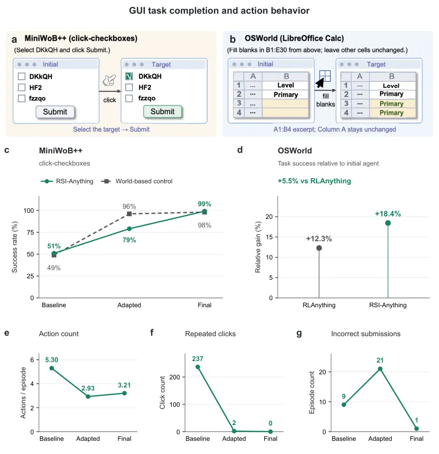
Figure 5: GUI evaluation (paper Figure 4). Panels a and b show initial and target states for the MiniWoB++ checkbox task and an OSWorld spreadsheet task; c gives click-checkboxes success for RSI-Anything and the World-based control across three configurations; d gives OSWorld success gain relative to the initial agent with the additional gain over RLAnything annotated; e to g give mean actions per episode, repeated clicks and incorrect-submission episodes for the configurations in c, with lines connecting only evaluated configurations.

Laboratory planning: five consecutive versions of a 4B policy

LabHorizon evaluates laboratory actions constrained by reagents, instruments and ordering. Level-1 is visually grounded next-action selection, Level-2 is protocol-aligned action-sequence generation, F200 is its 200-task setting, and the Level-2 Final Score combines action-sequence similarity with parameter accuracy. The authors follow five consecutive 4B policy versions from the same self-improvement process and evaluate them in development order on the same F200 Level-2 benchmark: 21.80%, 38.03%, 41.99%, 44.56%, 46.01%, with the last version 24.21 percentage points above the first. Evaluating in development order is the operational counterpart of the cycle index $k$: the version sequence is literally the set of retained pairs.

System	L1 accuracy	L2 Final
Grok 4.3	0.555	0.3244
Gemini 3.1 Pro	0.465	0.3263
GPT-5.5	0.535	0.2276
Kimi K2.6	0.550	0.3150
Qwen3.6-35B-A3B, direct prompting	0.475	0.2534
Qwen3.6-35B-A3B, trained	0.635	0.4100
Actor-Simulator-Selector reference	0.665	0.4532
RSI-Anything (4B)	0.700	0.4601

Table 5: reference systems and RSI-Anything on LabHorizon (paper Table 3). The reference orchestrates a trained Qwen3.6-35B-A3B Actor with Gemini 3.1 Pro as Simulator and Selector, and reports a Level-2 score of 0.4532.

Two observations carry weight. First, the reference is a three-model orchestration, a 35B Actor plus Gemini 3.1 Pro as Simulator and Selector, while RSI-Anything is a single 4B policy plus a protocol world model, and it wins 0.4601 to 0.4532 on Level-2, a margin of 0.69 percentage points, and 0.700 to 0.665 on Level-1. On this benchmark a small model with a consequence-predicting world model beats a large-model ensemble. Second, four frontier general-purpose models prompted directly land between 0.23 and 0.33 on Level-2, and the trained Qwen3.6-35B-A3B reaches 0.4100, still below the 4B RSI-Anything policy. The gap is not parameter count; it is whether a predictor trained for this protocol exists to screen candidate sequences.

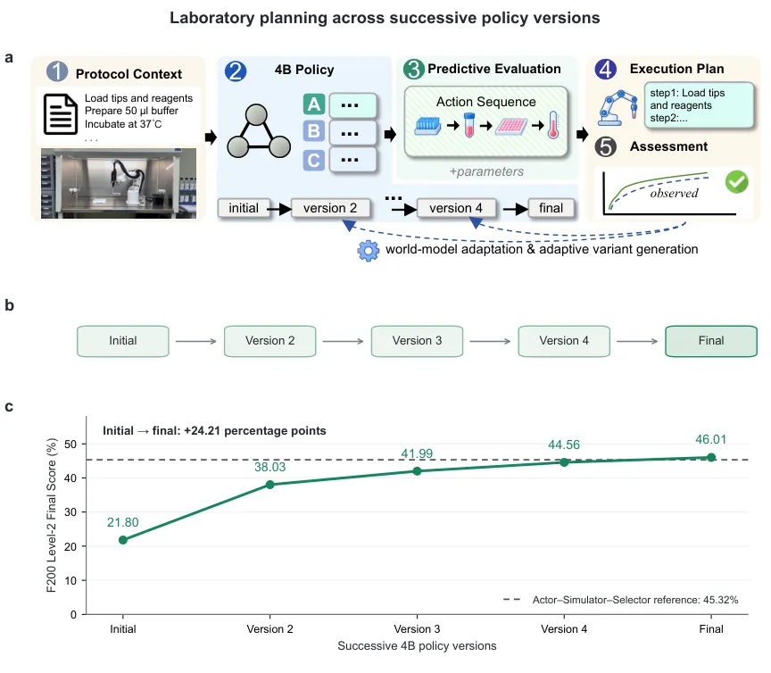
Figure 6: laboratory planning (paper Figure 5). Panel a sketches the planning workflow, protocol context into a 4B policy, predictive evaluation of action sequences and parameters, execution plan, evaluation, with dashed feedback paths marking the framework's update routes and the quantitative comparison below following retained policy versions. Panel b shows the five consecutive 4B versions from one self-improvement process and c their Final Scores, with a dashed line at the Actor-Simulator-Selector reference value of 45.32%; versions are ordered by development sequence and spacing is illustrative.

Reaction optimization: higher yield at a matched experiment count

The chemistry comparison is condition search at matched experiment counts. The adapter is ReactionT5-JEPA-Anything, which combines the ReactionT5 reaction-pretrained backbone with the JEPA-Anything predictive design, takes a serialized reaction $r$ and a candidate condition vector $c$, and outputs a predicted yield distribution $p_{\phi}\left(y\mid r,c\right)$. Two Suzuki-Miyaura screens are each compared against Bayesian optimization. The GC-analyzed screen varies a Pd-NHC-DMS precatalyst, base and solvent for the coupling of 4-chloroanisole with 4-(trifluoromethyl)phenylboronic acid; the flow LC-MS screen uses Pd(OAc)2 with ligand, base and solvent for substrates 1c and 2b. After 20 experiments the GC screen reaches a best observed yield of 93.0% against 87.5%, a gain of 5.5 percentage points; after 40 experiments the flow screen reaches a mean best observed yield of 96.15% against 82.16%, a gain of 13.99 percentage points. Each measured yield extends the observation history that guides the next condition choice, which is Equation 7's selection rule instantiated on a bench.

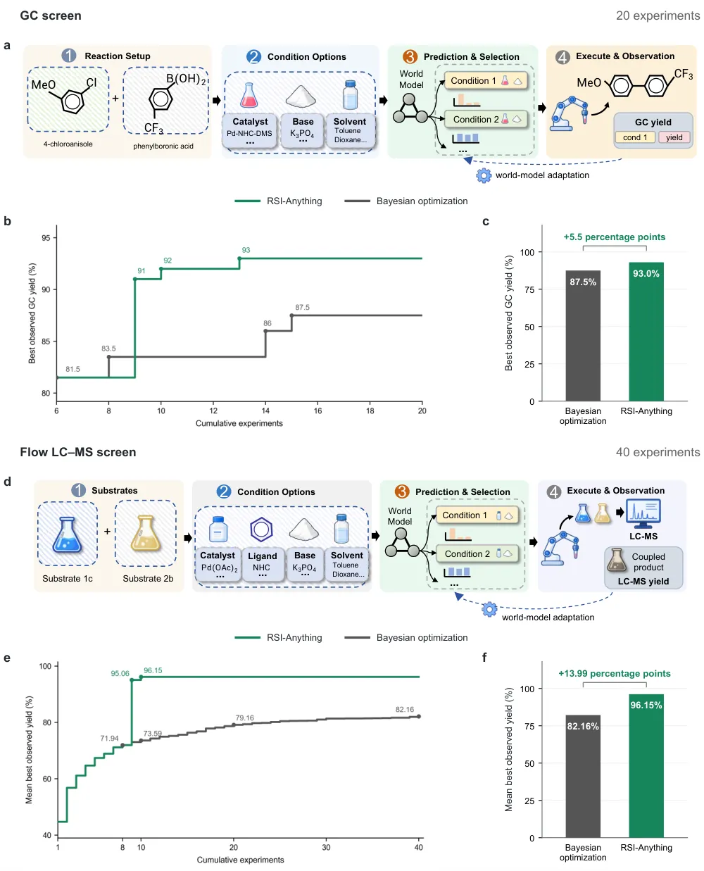
Figure 7: reaction-condition optimization (paper Figure 6; green RSI-Anything, gray Bayesian optimization). Panel a is the GC screen workflow from reaction setup through catalyst, base and solvent options to prediction-guided condition selection and measured yield; b and c give best observed GC yield against cumulative experiment count and the endpoint after 20 experiments; d is the flow screen workflow for substrates 1c and 2b with Pd(OAc)2, ligand, base and solvent followed by LC-MS analysis; e and f give the mean best observed yield curve and the endpoint after 40 experiments, with brackets marking the 5.5 and 13.99 percentage point gains.

The repository adds an evaluation detail the main text leaves thin. tasks/reaction_optimization/results/evaluation.json describes an offline sequential replay over measured screening yields with a candidate pool of 321 conditions, 100 runs seeded 4001 to 4100, eight starting observations and a total budget of 40. The pool optimum is itself 96.15%, and the mean final best observed yield across the 100 runs is also 96.15%, meaning every run reached the pool ceiling. By budget, the mean is 71.94% at observation eight, 80.14% at nine, and 96.15% from observation ten onward through forty; the first optimal hit has mean index 9.94 with median and maximum both ten. The companion validation.json records nine passing local inference unit tests, 3200 replayed recommendations, 4000 observed yields validated inside the evaluation environment, prediction arrays bit-identical to the sealed prior, and all reported metrics recomputed, alongside target_measurements_exported: false, i.e. the raw measurements themselves are not published with the repository.

Immune science: the same retention protocol applied to a research workflow

The final application is an end-to-end immune-science workflow connecting three things: persistent scientific-agent workflow development, predictive world-model construction, and evidence-guided analysis. During construction, Agent Genesis searches scientific-agent workflows and model configurations and selects a model-building agent workflow, which is the retained policy configuration for that stage, producing an action-conditioned immune world model that treats cytokines, genetic perturbations or candidate therapies as explicit actions and represents immune state at cellular, tissue and individual scales. During downstream analysis the world-model parameters are frozen while the analysis state, candidate interventions and hypothesis ranking evolve through model inference and self-correction; measured perturbation evidence supports modelling, and withheld interventions and biological contexts evaluate predictions and action composition.

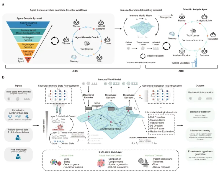
Figure 8: the end-to-end immune-science application (paper Figure 7). Panel A shows scientific-agent workflow evolution, immune world-model construction and model-guided analysis; panel B shows action-conditioned transitions over structured cellular, tissue and individual immune state with readouts used for interpretation, ranking and hypothesis generation. Panels A and B are adapted from Figure 1 of Cui et al. (2026a).

One result runs against intuition. During therapeutic hypothesis generation, self-correction removed all screened cytokine-pair candidates, and the integrated evidence produced a prospective nomination combining SIRP-alpha inhibition with IL-36-gamma-axis modulation, awaiting experimental testing. The output of this improvement round was therefore not a better-tuned version of the original hypothesis but the replacement of an entire hypothesis class, which is consistent with the framework's semantics: the retained workflow changed how subsequent candidates are generated, not merely how they are ranked. Evaluation details are deferred to Cui et al. (2026a) and are not repeated in this paper.

Limitations

The authors list four in the discussion. First, joint multi-round evaluation is still missing: in their words, joint multiround evaluation is needed to establish sustained mutual improvement of policy and world model within a single task. The current evidence is the two-stage gain from predictive selection plus predictor adaptation in code repair and the policy version sequence in laboratory planning, but no experiment runs full mutual improvement inside one task while reporting per-cycle accept and reject decisions. Second, the laboratory results assess protocol-aligned planning, and reliable physical execution still requires evaluation on the relevant equipment and workflows. Third, chemistry covers two Suzuki-Miyaura screens only, and holds only within the reported experiment budgets. Fourth, the therapeutic hypothesis from the immune-science application awaits experimental testing.

From a reviewer's seat, several more follow. First, each of the five experiments instantiates only part of the protocol, as paper Table 4 itself states: code repair fixes the policy, laboratory planning follows policy versions only, GUI updates both components but reports action-level diagnostics on a single task, chemistry measures feedback-guided search alone, and immune science separates construction from analysis. Evidence for the recursion claim is therefore assembled across experiments rather than established within one, and the paper never says in which experiments the pair gate of Equation 17 actually fired, how often, or with what rejection rate. Second, the 95% interval on the +2.83 percentage point code-repair gain has a lower bound of +0.17, barely above zero, and the capacity-matched static verifier is the authors' own construction, so how thoroughly it was tuned cannot be judged from the text. Third, the five laboratory versions were evaluated in development order on F200, and F200 is also their development feedback source; the paper requires a held-out audit set for final reporting but does not disclose whether gate data for these five versions was strictly separated from F200, so how much of the monotone climb is adaptation to this benchmark and how much is genuine planning improvement cannot be separated from the available information. Fourth, the reliability trichotomy of Equation 10 has no published thresholds in any domain, for error, calibration, drift or coverage, so a reproducer cannot tell when $u_{k}^{W}$ would be set to one; the repository goes further and states calibration_verified: false and semantic_correctness_guaranteed: false in the semantic_world.py manifest, meaning the calibration of those five-class probabilities was never verified. Fifth, GUI success comes from 100 test instances with no seeds or intervals reported, and OSWorld gives relative gains without absolute success rates or confidence intervals, so a reader cannot tell how many tasks 18.4% corresponds to. Sixth, the chemistry result of 96.15% equals the pool optimum over 321 candidates exactly, so the metric saturates at the pool ceiling and the 13.99 percentage point advantage over Bayesian optimization measures search efficiency rather than discovery ability; it is also an offline sequential replay whose raw measurements are not released. Seventh, reproducibility is tiered: code repair and GUI have complete runnable workflows and configs, laboratory planning and reaction optimization have inference-side adapters with sealed results, and immune science has documentation only.

Conclusion and Outlook

The durable contribution here is not a model but a protocol that writes prediction and retention as the two ends of one formalism. Prediction decides who spends external feedback (Equations 7 and 8), feedback decides what gets updated (Equations 9 and 12), reliability decides when the predictor may be updated at all (Equations 10 and 11), and the component plus pair gates decide which pair is retained (Equations 13 to 18). Four design choices are worth memorizing separately: reliability is three-valued, so thin coverage is not reliability; predictions must be attributable to the current model version, so older predictions never contaminate the present error estimate; training admission and external evaluation selection are governed separately, so refusing to train on a record does not mean refusing to experiment on it; and a failed pair check rolls both components back rather than one. Taken together these are exactly the parts that get dropped when a system has to cope with the coupling problem, namely that changing the policy changes the distribution on which the predictor is judged.

The distribution of evidence is equally clear. Predictive selection plus predictor adaptation gives two successive gains in code repair while online usage stays flat, so the gain is not bought with extra test budget. In GUI work, three retained configurations improve success and action economy together, and the middle configuration doubles as a demonstration of how a single metric misleads. In laboratory planning a 4B policy with a protocol world model beats a three-model orchestration. In chemistry the same experiment count buys a higher yield. The next step is the one the authors name themselves: run full joint multi-round improvement of policy and model inside a single task and report gate decisions and acceptance rates per cycle. Then publish the reliability thresholds and calibration results, without which conditional adaptation cannot be reproduced in anybody else's laboratory. Third, bring physical execution and real equipment into the laboratory evaluation so that a 46.01% planning score can be connected to bench success. For anyone building agent runtimes, the transferable part is not the model architecture but the three-way data discipline of update data, gate data and a held-out audit set, plus the insistence on aligned state signatures as a precondition for paired comparison.

Golden Quote

"Update the policy and the candidate and experience distributions the world model depends on change with it; update the model and ranking, imagined trajectories and learning signals all change too. Improving either component therefore does not guarantee that the assembled system improves, which is why retention has to be treated as a first-class operation."