SimpleVLN: Towards Simple and Frontier Vision-Language Navigation

Paper Metadata

Title: SimpleVLN: Towards Simple and Frontier Vision-Language Navigation

Authors: Lingyi Hong, Weiren Cai (co-first authors), Jiayu Chen, Xinyu Zhou, Bailin He, Yunfei Guo, Qiao Sun, Boyu Ma, Jianfei Yang, Wenqiang Zhang (Fudan University, Nanyang Technological University, Lenovo Research; the author list marks co-project leads and a corresponding author)

Links: arXiv:2610.23203 (v1, 2026-10-16, cs.RO) · arXiv HTML full text · project page · GitHub · HuggingFace weight collection

Code status: ✅ partially released. github.com/simplevln/SimpleVLN publishes the full evaluation path: a 687-line eval/vln/eval.py (navigation agent over a Habitat environment plus a vLLM OpenAI-compatible endpoint), val_unseen annotation packs for R2R-CE and RxR-CE (1839 and 3669 episodes), Matterport3D scene preparation scripts, two Hydra configs, resumable result storage, and eight SFT and RL checkpoints spanning Qwen2.5-VL 3B/7B, Qwen3-VL 4B/8B and Qwen3.5 4B/9B. ⛔ The training side is not there: no IL/DAgger/RL training scripts, no RL task-synthesis pipeline, no DAgger deviation threshold, and the repository declares no license (only a CC-BY-4.0 note inside the data directory plus MP3D access instructions). The repo was created 2026-10-15, last pushed 2026-10-19, and has 10 stars. What the public code reproduces is therefore "how to evaluate", not "how the 76.7% was trained".

Background and Motivation

Vision-language navigation asks an embodied agent to follow a natural-language instruction through an environment it has never seen: turn "go down the hall, take the second door on your left, stop by the sofa" into first-person pixels, and keep the decisions consistent over tens or hundreds of steps. VLN-CE moves this task from predefined discrete viewpoints into continuous environments, where actions are decomposed into low-level primitives (forward 0.25 m, turn 15 degrees left or right, stop). Long-horizon decision making, error accumulation and observation organization then all become real problems at once.

Most of the progress in recent years came from task-specific structure. One family augments perception and spatial reasoning, as JanusVLN does with a 3D geometry encoder. Another builds explicit graph representations, abstracting the environment into a topology and deciding over it. A third goes hierarchical or dual-system: DualVLN, SEDualVLN, AgentVLN and NavFoM split reactive control from deliberative planning across two modules. StreamVLN introduces a streaming context, and a further line of work attaches explicit chain-of-thought reasoning to the model. These designs did push scores up, but they also hid a question: in any single evaluation, how much of the score comes from the backbone MLLM and how much from the modules bolted onto it?

The authors argue that this attribution is currently impossible. An augmented system's performance reflects the backbone and the task module together, so "how far can a native MLLM walk on its own" has never been measured in isolation. The paper turns that into an explicit question: before introducing task-specific architecture, have we actually exhausted what a native MLLM can do on VLN? To answer it honestly, the authors impose a hard constraint on themselves: do not touch the architecture. No graph encoder, no memory module, no dual system, no change to the forward pass. What remains editable is what goes in, what comes out, what data trains it, and what objective trains it.

Preserving the architecture is not the same as doing nothing. Turning a model pretrained for image-text question answering into a policy that walks continuously requires at least three things to be redone, and those are the three axes of SimpleVLN. The formulation axis decides what one decision sees and says: single-turn reconstructed input with a fixed-budget global-local memory keeps the context from growing without bound over an episode, and action chunks let one inference emit several primitive actions. The data axis decides where supervision comes from: expert demonstrations give action-level supervision, deviation-based DAgger adds the states the policy actually reaches, and the RL stage widens the distribution with automatically synthesized tasks. The optimization axis decides what is being optimized: imitate actions, then correct on the policy's own state distribution, then optimize task-level success directly.

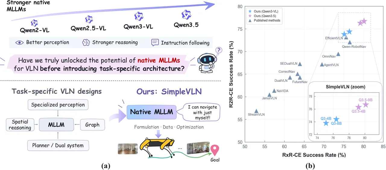
Figure 1: paper Figure 1. (a) Motivation - the score of an augmented MLLM system mixes two contributions, the backbone and the task modules, so native MLLM navigation ability has never been measured on its own. (b) Success-rate comparison on R2R-CE and RxR-CE val-unseen: SimpleVLN pushes both benchmarks to the front using monocular RGB only.

The answer up front: this "change only the interface, the data and the objective" recipe beats existing methods that use panoramas, depth or dual systems on both benchmarks, and backbone upgrades convert straight into gains - the same pipeline moves from 51.6% on Qwen2.5-VL 3B to 76.7% on Qwen3.5-9B. That is the practical dividend of keeping the architecture: a better base model does not require redesigning the navigation system.

Preliminaries

The VLN-CE setting and its metrics. Environments are real indoor scans from Matterport3D running in Habitat. The action space is discretized as $\mathcal{A}=\{\text{Forward}(0.25\,\text{m}),\ \text{TurnLeft}(15^{\circ}),\ \text{TurnRight}(15^{\circ}),\ \text{Stop}\}$; an episode ends when Stop is executed or the primitive-action budget $S_{\max}$ runs out, and stopping within 3 m of the goal counts as success. Each of the five metrics measures one thing. NE is the straight-line distance from the final position to the goal (lower is better). OS records whether the trajectory ever entered the success radius. SR is success rate, the headline metric of this paper. SPL weights success by the ratio of reference path length to actual path length, so detours are penalized. nDTW measures shape similarity to the reference path. The gap between SPL and SR therefore reads as "arrived, but wastefully".

What "architecture-preserving" means concretely. SimpleVLN uses an off-the-shelf MLLM (Qwen2.5-VL, Qwen3-VL or Qwen3.5) through an OpenAI-compatible chat interface served by vLLM. One decision is one multi-image chat request: a system prompt, the instruction text, and several base64 JPEG frames; the response is text, and the action is parsed out of that text. Beyond the weights, the whole system consists of prompt assembly, image sampling and text parsing. There is no new learnable module anywhere, which is exactly why it can consume an existing inference stack and why it improves when the backbone improves.

How the three training paradigms divide the work. Imitation learning extracts actions from expert trajectories, and pays for it with distribution shift: once the policy errs into a state no expert ever visited, the supervision stops applying. DAgger answers this by collecting expert labels on the states the policy itself induces. RL takes the task-level outcome as the signal and no longer requires the action sequence to match a reference. Supervision granularity gets coarser while the objective gets more honest: from "is this action right", to "what should I do where I actually end up", to "did the task succeed". SimpleVLN chains the three into one progressive pipeline instead of picking one.

Method

Notation: separating environment steps from decision steps

The first engineering decision is a redefinition of the time axis. Given a natural-language instruction $\mathcal{I}$, at the $k$-th primitive environment step the agent observes an egocentric RGB image $x_k$ and executes $u_k\in\mathcal{A}$. The model, however, is not called at rate $k$ but at decision steps $t=1,2,\dots$. Let $n_t$ be the number of primitive actions executed before decision $t$ (with $n_1=0$); then the current observation is $o_t=x_{n_t}$, and one decision may span several primitive steps. The entire formulation layer is written in terms of $t$, which is what later makes action chunks and a memory budget self-consistent.

Single-turn decision input: rebuild every step, never accumulate

The most counter-intuitive choice is that SimpleVLN does not append the new observation and the previous prediction to an existing conversation. Every decision builds one independent turn from scratch, containing only the instruction $\mathcal{I}$, the current observation $o_t$ and the sampled visual history $H_t$. Previous turns and previously executed actions never enter the context. The visual part of that turn is written $s_t=(o_t,H_t)$.

The justification comes straight from the ablation (Table 3(b)): multi-turn accumulation scores 35.7% SR, single-turn reconstruction scores 53.6%, a gap of 17.9 points. The authors' reading is that although a multi-turn conversation preserves a more complete interaction history, continuously appending observations and actions creates an over-long context that current MLLMs cannot use effectively for navigation. In other words, on these models "remembering more" is not "using it better"; compressing the context into a fixed-shape decision snapshot is easier for the model to exploit.

Global-local memory: compressing history under a fixed budget

Since history does not go into the conversation, it needs somewhere else to live. By decision $t$ the primitive-step observation sequence $(x_0,\dots,x_{n_t-1})$ keeps growing with interaction: keeping all of it explodes the input, keeping only the last few frames discards the earlier route context. SimpleVLN represents history on two complementary time scales - a local history for recent continuity and a global history that sparsely covers older observations:

$$L_{t}=(x_{k})_{k=\max(0,\,n_{t}-N)}^{\,n_{t}-1},\qquad m_{t}=\min\{M,\ \max(0,\,n_{t}-N)\} \tag{1}$$ $$G_{t}=(x_{i_{j}})_{j=1}^{m_{t}},\qquad H_{t}=G_{t}\,\|\,L_{t}$$

Here $\|$ is sequence concatenation, $L_t$ takes at most $N$ frames immediately preceding $o_t$, and $G_t$ samples at most $M$ frames uniformly from the older history. When $m_t>0$, the sampled indices satisfy $0\leq i_{1}<\dots<i_{m_{t}}<\max(0,n_{t}-N)$. The property that matters is the fixed budget: whether the episode lasts 40 steps or 400, the number of frames entering the model is capped at $M+N+1$, so context length does not grow with time. Streaming-context approaches such as StreamVLN solve the same problem, but by compressed encoding rather than by resampling.

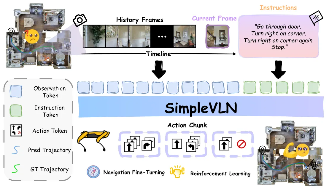
Figure 2: paper Figure 2, SimpleVLN overview. Each decision assembles the sampled history frames, the current observation and the instruction into one turn for the MLLM, and the model directly predicts an action chunk used for navigation - with no additional module in between.

The budget is not guessed, it is swept (paper Figure 4). Fixing $N=1$ and varying $M$: SR peaks at $M=8$ and then falls as the global budget keeps growing, which indicates that excessive global history introduces redundant or irrelevant observations and dilutes the useful context. Fixing $M=8$ and varying $N$: a single local frame is best, and additional neighbouring frames are mostly repeated information. The default configuration is therefore $M=8$, $N=1$ - at most 8 global frames plus 1 local frame plus the current observation, 10 frames in total.

Action chunks: one decision says several actions

The output representation changes as well. Following NaVIDA, SimpleVLN has each decision predict an action chunk $a_t$, an ordered sequence of primitive actions. With $K_t$ primitives in the chunk, $a_{t}=(u_{n_{t}},\dots,u_{n_{t}+K_{t}-1})$, and the policy is written

$$a_{t}\sim\pi_{\theta}\big(\cdot\mid\mathcal{I},s_{t}\big)=\pi_{\theta}\big(\cdot\mid\mathcal{I},o_{t},H_{t}\big)$$

where $\pi_\theta$ is the native MLLM itself. The environment executes the chunk in order, each step produces one observation and all of them are retained for building later histories; the model is queried again only after the chunk finishes, unless Stop or the primitive budget $S_{\max}$ ends the episode first. This design pays off twice. Fewer model calls is the obvious part, but the ablation (Table 3(a)) shows it is also the better output representation: predicting one primitive action per call gives 45.6% SR, switching to action chunks gives 53.6%, a net 8.0 points. The authors explicitly frame it as a formulation-level improvement, not merely a compute saving.

Data construction: demonstrations, corrections, synthesis

Expert demonstration coverage. Trajectories from R2R, RxR and ScaleVLN are pooled to broaden the coverage of expert behaviour, and each is converted into decision-level samples that match the inference interface exactly: input $(\mathcal{I},s_t)$, target the corresponding expert action chunk $a_t^{\star}$. Training and inference share one shape, and that is what later lets DAgger and RL data mix straight in.

Policy-relevant experience (DAgger). Broader demonstrations do not remove the distribution gap between expert trajectories and the states the policy actually visits. The authors use a deviation-based DAgger rule: compare the current policy trajectory against the ground-truth trajectory, take the expert trajectory when the deviation is large and keep the policy trajectory otherwise; selected trajectories are converted into decision-level samples and aggregated with the demonstration data. This is the single largest item in Table 4 (+7.5 SR on R2R-CE, +8.1 on RxR-CE), which says that supervising the model where it actually goes is worth more than showing it yet more expert routes.

RL task synthesis. At the RL stage, reusing the episodes already consumed by supervised learning would neither widen the task distribution nor provide genuinely new interaction experience, so the authors synthesize new tasks inside the training scenes: start-goal pairs are sampled from the navigation graph with the two endpoints in different rooms, the goal bound to a semantically annotated object; an MLLM then generates the navigation instruction from the reference path's waypoints (turns, rooms, salient objects, first-person views). The reference path is used only to construct the task and never as an action target, and val-unseen scenes are excluded. This pipeline removes the human-annotation ceiling on RL data volume.

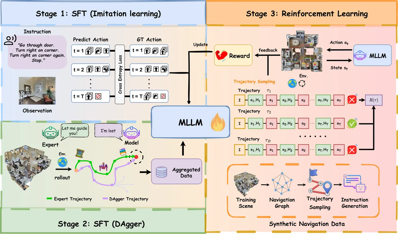
Figure 3: paper Figure 3, the training data pipeline. The agent first learns from expert demonstrations, then DAgger collects and aggregates correction trajectories; at the RL stage, navigation episodes are synthesized from sampled start-goal paths with generated instructions, and the policy is optimized through environment interaction and outcome feedback.

Progressive optimization: from imitating actions to optimizing outcomes

Stage one, imitation learning. Let the supervised set $\mathcal{D}$ consist of triples $(\mathcal{I},s_t,a_t^{\star})$. The objective minimizes the negative log-likelihood of the entire target action chunk:

$$\mathcal{L}_{\mathrm{SFT}}=-\mathbb{E}_{(\mathcal{I},s_{t},a_{t}^{\star})\sim\mathcal{D}}\Big[\log\pi_{\theta}\big(a_{t}^{\star}\mid\mathcal{I},s_{t}\big)\Big] \tag{2}$$

Note that the likelihood is taken over the whole chunk rather than weighting each primitive action independently - this is what pairs with the action-chunk output representation. Stage two, DAgger adaptation. The objective $\mathcal{L}_{\mathrm{SFT}}$ is unchanged word for word; only $\mathcal{D}$ changes, gaining the target action chunks of the policy-relevant trajectories selected above. Stage three, reinforcement learning. The policy interacts with the environment on synthesized episodes, predicting an action chunk per decision and forming the trajectory

$$a_{t}\sim\pi_{\theta}\big(\cdot\mid\mathcal{I},s_{t}\big),\qquad \tau=\big((s_{t},a_{t})\big)_{t=1}^{T} \tag{3}$$

where $T$ is the number of model-level decisions actually taken before the episode terminates, which is not the same quantity as the primitive budget $S_{\max}$. The reward is a binary task-level signal, with the success criterion inherited from the stopping and distance conditions in Section 3.1:

$$R(\tau)=\mathbb{I}(\mathrm{success})\in\{0,1\},\qquad \max_{\theta}\ \mathcal{J}_{\mathrm{RL}}(\theta)=\mathbb{E}_{\tau\sim p_{\theta}}\big[R(\tau)\big] \tag{4}$$

The meaning of a binary reward deserves unpacking: it does not require the trajectory to match any reference action sequence, so any route that succeeds earns full credit. For a task where one instruction admits several reasonable paths, this injects less human preference than a shaped reward, and the experiments agree (Table 6: SPL reward 68.9 versus binary success reward 70.1, R2R-CE SR). The learning signal thus makes a three-step jump: expert action supervision, then policy-relevant supervised adaptation, then episode-level task-completion feedback.

Training configuration. Backbones are Qwen3-VL (4B/8B) and Qwen3.5 (4B/9B). The IL stage runs SFT for 3 epochs on R2R and RxR with a frozen vision encoder and peak learning rate $2\times10^{-5}$; training then continues for 1 epoch on the collected DAgger data and 2 more epochs on the mixture with ScaleVLN. RL for the main results uses DAPO for 40 steps with batch size 256, 16 rollouts per prompt, learning rate $1\times10^{-6}$, KL coefficient 0 and clip ratios 0.30/0.20. Forty RL steps buying 7.5 to 10.2 SR points is the highest-yield segment in the paper.

Method to source code

The public repository covers evaluation only, but it happens to implement all three formulation-layer designs in readable code. Correspondence one: uniform sampling of the global memory. The "at most $M$ frames sampled uniformly" of $G_t$ in Equation (1) is an endpoint-inclusive equidistant index function in eval/vln/eval.py, called with $M$ hard-coded to 8 and deliberately excluding the current frame (rgb_list[:-1]):

# eval/vln/eval.py:168
def uniform_sample_with_ends(self, data, n):
    if len(data) <= n:
        return data
    indices = [round(i * (len(data) - 1) / (n - 1)) for i in range(n)]
    return [data[i] for i in indices]

# eval/vln/eval.py:312,329  single-turn rebuild + 8 global frames + current observation
self.conversations = self.conversations[:1]          # keep only the system message
content.extend([{"type": "image_url", ...} for item in
                self.uniform_sample_with_ends(self.rgb_list[:-1], 8)])
content.append({"type": "image_url", ...encode_image_base64(self.rgb_list[-1])})

The line self.conversations[:1] is the entire implementation of "single-turn decision input": each step truncates the conversation back to the system prompt (SYSTEM_PROMPT = "You are a visual language navigation model.") and re-assembles one user turn. The fixed budget of the observation buffer is enforced by --max-action-history (default 10) - anything beyond it drops the oldest frame, which is exactly $M+N+1=8+1+1$.

Correspondence two: parsing and expanding the action chunk. The model output is comma-separated sub-action text; extract_multi_result() splits on ', ', extract_result() strips <answer>...</answer>, classifies stop / forward / left / right by keyword and regexes one number out of the text as a magnitude. Magnitude-bearing outputs (for example "forward 0.75", "left 30") are then expanded into primitives, at most 3 per sub-action:

# eval/vln/eval.py:344-368
select_action_idx = 2
result = result[:select_action_idx]                # keep only the first two sub-actions
for action_index, numeric in result:
    if action_index == 1:                          # forward
        for _ in range(min(3, round(numeric / self.forward_distance))):
            self.pending_action_list.append(1)
    elif action_index == 2:                        # turn left
        for _ in range(min(3, round(numeric / self.turn_angle))):
            self.pending_action_list.append(2)
    if action_index is None or len(self.pending_action_list) == 0:
        action_index = random.randint(1, 3)        # random fallback on parse failure
        self.pending_action_list.append(action_index)

Pending actions queue up in pending_action_list and act() pops one per step; the model is not called while the queue is non-empty - precisely the paper's "query the MLLM again only after the chunk finishes". Correspondence three: environment constants. eval/config/vln_r2r.yaml sets forward_step_size: 0.25, turn_angle: 15, success_distance: 3.0, max_episode_steps: 400 and RGB 640x480 with hfov 90, matching the action space and success criterion of Section 3.1 item by item. A depth sensor is defined in that config, yet the agent reads only observations["rgb"], consistent with the monocular-RGB-only claim.

flowchart TB
    subgraph LOOP["Decision loop at inference - architecture unchanged"]
        E["Habitat primitive step k
egocentric RGB x_k"] --> B["Observation buffer
drop oldest beyond max_action_history = 10"]
        B --> G["Global memory G_t
8 frames uniform with ends"]
        B --> L["Local memory L_t
N = 1 recent frame"]
        I["Instruction I"] --> C["Rebuild single-turn context
system prompt + I + G_t + L_t + o_t"]
        G --> C
        L --> C
        C --> M["Native MLLM pi_theta via vLLM
no extra encoder, no memory module"]
        M --> A["Action chunk a_t
comma separated sub-actions"]
        A --> P["Parse and expand
first 2 sub-actions, at most 3 primitives each"]
        P --> Q["pending_action_list"]
        Q --> X["Execute Forward 0.25 m / Turn 15 deg / Stop"]
        X --> E
    end
    subgraph TRAIN["Progressive optimization IL - DAgger - RL"]
        D1["Expert demos pooled
R2R + RxR + ScaleVLN"] --> S1["Stage 1 IL
SFT on full chunk likelihood, 3 epochs, frozen vision encoder"]
        S1 --> D2["Deviation-based DAgger
policy trajectory vs GT trajectory"]
        D2 --> S2["Stage 2 DAgger SFT
same loss, 1 epoch then 2 epochs with ScaleVLN"]
        SY["Task synthesis
start-goal pairs in train scenes + MLLM instructions"] --> S3["Stage 3 RL
DAPO 40 steps, batch 256, 16 rollouts"]
        S2 --> S3
        S3 --> RW["Binary reward R = 1 if stopped within 3 m else 0"]
        RW --> S3
    end
    S2 -. IL-DAgger checkpoint .-> M
    S3 -. RL weights .-> M

Figure 4: the two loops of this method, drawn from Sections 3.2-3.4 of the paper and the public evaluation code. The top half is the inference decision loop: buffer, global/local sampling, single-turn reconstruction, native MLLM, action-chunk parsing, sequential execution. The bottom half is the three-stage progressive training, where IL and DAgger share the likelihood objective of Equation (2) and RL switches to the binary outcome reward of Equation (4). Dashed arrows denote weight hand-off.

Experimental Results

Evaluation runs on Matterport3D inside Habitat and reports the val-unseen splits of R2R-CE and RxR-CE with NE, OS, SR, SPL and nDTW, SR being primary. Table 1 is the main comparison: SimpleVLN uses monocular RGB only, yet beats methods that use panoramas, depth or dual systems on both benchmarks simultaneously.

Method	Size	Observation	R2R NE↓	R2R SR↑	R2R SPL↑	RxR SR↑	RxR nDTW↑
NaVid	7B	monocular RGB	5.47	37.4	35.9	23.8	-
Uni-NaVid	7B	monocular RGB	5.58	47.0	42.7	48.7	-
NaVILA	7B	monocular RGB	5.22	54.0	49.0	49.3	58.8
StreamVLN	7B	monocular RGB	4.98	56.9	51.9	52.9	61.9
JanusVLN	7B	monocular RGB	4.78	60.5	56.8	56.2	62.1
NaVIDA	3B	monocular RGB	4.32	61.4	54.7	57.4	67.0
DualVLN	7B	monocular RGB	4.05	64.3	58.5	61.4	70.0
CorrectNav	7B	monocular RGB	4.24	65.1	62.3	69.3	75.2
SEDualVLN	7B	monocular RGB	3.75	67.3	62.5	63.9	72.8
AgentVLN	3B	RGB + depth	3.88	67.2	64.7	69.5	74.6
OmniNav	3B	panorama	3.74	69.5	66.1	73.6	-
Qwen-RobotNav	8B	panorama	3.53	72.1	66.6	76.5	72.5
Efficient-VLN	8B	monocular RGB	3.29	73.2	65.0	75.6	-
SimpleVLN† Qwen2.5-VL	3B	monocular RGB	5.70	51.6	44.9	50.3	57.6
SimpleVLN† Qwen3-VL	4B	monocular RGB	4.26	65.4	58.8	63.4	66.5
SimpleVLN* Qwen3-VL	4B	monocular RGB	3.39	73.8	66.7	75.1	71.5
SimpleVLN* Qwen3-VL	8B	monocular RGB	2.93	74.4	69.5	76.4	77.4
SimpleVLN* Qwen3.5	4B	monocular RGB	2.79	76.3	72.3	79.2	80.3
SimpleVLN* Qwen3.5	9B	monocular RGB	2.63	76.7	72.6	80.1	79.8

Table 1: main comparison on R2R-CE and RxR-CE val-unseen (selected from paper Table 1; † before RL, * after RL). The observation column separates monocular RGB, RGB plus depth, and panorama - every SimpleVLN row uses monocular RGB only, with no odometry and no depth. NE is in metres, the rest in percent.

Three things can be read out of the table. First, sensors are not the source of the gap: Qwen-RobotNav 8B with panoramas scores 72.1, AgentVLN 3B with depth scores 67.2, while SimpleVLN 4B (73.8) already passes Efficient-VLN 8B (73.2) and the 9B variant lifts R2R-CE to 76.7 and RxR-CE to 80.1. Second, RL helps consistently on every backbone: Qwen3-VL 4B goes from 65.4 to 73.8 on R2R-CE and from 63.4 to 75.1 on RxR-CE, and the four RL checkpoints in the repository are reported as +7.5 to 10.2 points on R2R-CE and +11.7 to 16.1 on RxR-CE. Third, backbone upgrades convert directly into navigation scores: the same pipeline runs from 51.6 on Qwen2.5-VL 3B to 76.7 on Qwen3.5-9B with no structural change in between - the most concrete payoff of preserving the architecture.

Method	Size	Latency per decision (ms)↓	R2R-CE SR↑	RxR-CE SR↑
StreamVLN	7B	300	56.9	52.9
DualVLN	7B	683	64.3	61.4
JanusVLN	7B	906	60.5	56.2
FutureNav	4B	1141	65.4	60.9
SimpleVLN (Qwen3-VL)	4B	293	73.8	75.1

Table 2: inference latency versus performance (paper Table 2). Measured on the same NVIDIA A100, counting only model execution time for one action-chunk decision, excluding preprocessing, environment execution and other non-model overhead.

The latency column matters because cheap here does not mean compromised. At 293 ms SimpleVLN matches the streaming baseline StreamVLN (300 ms), runs 2.3 times faster than the dual-system DualVLN (683 ms) and 3.9 times faster than FutureNav (1141 ms), while scoring 8.9 to 16.9 SR points higher. The reason is not mysterious: the context is a fixed 10-frame single turn, so prefill length does not grow with the episode; the output is an action chunk of a few tokens, so decoding is short; and one decision can drive up to 6 primitive steps, lowering the inference cost amortized per step.

Ablation group	Variant	NE↓	OS↑	SR↑
Action format	primitive actions (1 per decision)	5.2	54.5	45.6
	action chunk (default)	5.5	61.2	53.6
Conversation format	multi-turn accumulation	5.9	55.2	35.7
	single-turn reconstruction (default)	5.5	61.2	53.6
Observation sampling	sample chunk boundaries only	6.1	55.2	46.3
	keep every primitive frame	5.8	57.5	51.9
	8 global frames, uniform (default)	5.5	61.2	53.6

Table 3: the three formulation-layer ablations (paper Tables 3(a)(b)(c)), all with Qwen3-VL 4B fine-tuned on R2R and evaluated on R2R-CE val-unseen; bold marks the SimpleVLN default. The "8 frames" row of observation sampling covers the global history only, excluding the local frame and the current observation.

The formulation ablations carry the highest information density in the paper. The +17.9 SR of single-turn reconstruction over multi-turn accumulation is the largest single gap, which says current MLLMs use long conversational navigation context very poorly; the +8.0 SR of action chunks rules out the "it only saves calls" explanation. The observation-sampling group is the interesting one: sampling chunk boundaries only (46.3) is worse than keeping every primitive frame (51.9), and sampling 8 global frames uniformly (53.6) beats "keep everything" by 1.7 points. More observations act as noise here, not information.

R2R	RxR	ScaleVLN	DAgger	R2R NE↓	R2R OS↑	R2R SR↑	R2R SPL↑	RxR SR↑	RxR SPL↑	RxR nDTW↑
✓				5.53	61.2	53.6	48.1	50.3	42.0	57.6
✓	✓			5.28	63.4	56.7	51.3	54.5	46.7	62.4
✓	✓	✓		4.90	68.4	57.9	50.9	55.3	48.1	63.6
✓	✓	✓	✓	4.26	74.3	65.4	58.8	63.4	54.1	66.5

Table 4: demonstration and DAgger data ablation (paper Table 4), Qwen3-VL 4B, R2R-CE and RxR-CE val-unseen.

The data-side arithmetic is equally clean. Adding RxR moves R2R-CE SR from 53.6 to 56.7 and RxR-CE from 50.3 to 54.5, an in-domain gain; adding ScaleVLN takes them to 57.9 and 55.3, improving generalization to unseen environments; DAgger alone then delivers +7.5 on R2R-CE and +8.1 on RxR-CE, the largest item in Table 4, while NE drops from 4.90 to 4.26 and OS rises from 68.4 to 74.3. What it fixes is not "occasionally right" but "drifts less".

RL configuration	R2R NE↓	R2R OS↑	R2R SR↑	R2R SPL↑	RxR SR↑	RxR SPL↑	RxR nDTW↑
pre-RL baseline	4.26	74.3	65.4	58.8	63.4	54.1	66.5
synthesis scene pool: R2R only	3.91	74.0	68.5	63.2	65.8	55.3	68.3
synthesis scene pool: RxR only	3.76	71.8	67.5	59.3	68.5	59.5	68.8
synthesis scene pool: ScaleVLN only	4.17	70.9	66.6	61.3	66.3	56.2	67.3
synthesis scene pool: R2R + RxR + ScaleVLN	3.74	73.1	70.1	65.6	71.0	62.1	68.4
GRPO + SPL(τ) reward	3.80	73.9	68.9	63.1	67.7	58.3	67.3
GRPO + binary success reward	3.74	73.1	70.1	65.6	71.0	62.1	68.4
DAPO + binary success reward	3.45	76.6	71.5	65.3	73.7	64.0	69.4

Table 5: RL data and configuration (paper Tables 5 and 6 merged), Qwen3-VL 4B. The scene-pool rows and both GRPO rows use batch 32 with 8 rollouts per prompt; the main-result configuration uses DAPO, batch 256 and 16 rollouts per prompt.

The RL section yields three actionable conclusions. First, mix the scene sources of synthesized tasks: the three pools used alone reach 68.5 / 67.5 / 66.6 (R2R-CE SR), while the mixture reaches 70.1 with 71.0 on RxR-CE, both above the pre-RL baseline. Second, simpler reward is better: SPL-shaped reward gives 68.9, binary success reward 70.1 (RxR-CE 67.7 to 71.0), supporting "ask only whether the task succeeded". Third, the optimizer has a visible effect: with the reward fixed to binary, DAPO reaches 71.5 / 73.7 while GRPO reaches 70.1 / 71.0. The training dynamics (paper Figure 5) agree: rollout reward and evaluation SR both trend upward while the average number of decisions per trajectory declines - RL makes the agent not just more accurate but more decisive, finishing the same route with fewer model calls.

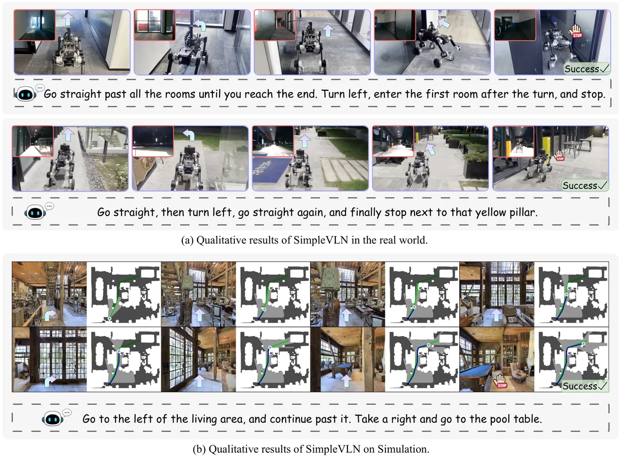
Figure 5: paper Figure 6, SimpleVLN in simulation and in the real world. It follows several different instructions to the designated goal; arrows show the navigation direction.

The hardware section gives a complete sim-to-robot path: the model runs on a Daystar quadruped, compute is an onboard NVIDIA Jetson Thor, perception comes from an Intel RealSense D450 RGB-D camera but only the RGB channel is used as observation. The paper reports that it follows multi-step instructions containing forward motion, turns, entering rooms and stopping at landmarks, and that it maintains coherent instruction-following over longer trajectories. For a discrete action space of 0.25 m and 15 degrees, closing the loop on onboard compute is itself a meaningful engineering result - it means the method does not depend on an offline GPU server.

Limitations

Stated by the authors, first: the memory budget is non-monotonic and the optimum is found by sweeping. Paper Figure 4 shows that with $N=1$ fixed, SR peaks at $M=8$ and then falls as the global budget grows; the authors attribute this to excessive global history introducing redundant or irrelevant observations that dilute the useful context, and with $M=8$ fixed, keeping more local frames brings no gain either. "Looking at more" therefore does not hold under this input organization, but the paper offers only one empirical optimum, with no rule for adapting the budget to scene scale, instruction length or episode length. Whether $M=8$ remains optimal in an environment with a different distribution of building sizes is unknown.

Stated by the authors, second: the RL gain cannot be attributed to the optimizer alone. The +1.4 / +2.7 SR of DAPO over GRPO in Table 6 was measured in the ablation setting of batch 32 with 8 rollouts per prompt, whereas the main results use batch 256 with 16 rollouts. The authors write explicitly that they do not attribute this gain solely to the optimization algorithm. The conclusion "DAPO is better" is thus coupled to its specific hyperparameters and cannot be lifted out directly.

Stated by the authors, third: real-robot evaluation is qualitative only. Section 4.6 gives the success cases and direction arrows of Figure 6, with no real-world success rate, no instruction count, no failure-mode statistics and no onboard inference latency. The 293 ms of Table 2 is an A100 number; how long one decision takes on a Jetson Thor and whether it can keep up with the quadruped gait are questions the paper does not answer.

My reading, first: a backbone baseline is missing, and it is exactly the answer to the question in the title. The paper repeatedly asks whether the potential of native MLLMs has been exhausted, yet reports no VLN score for Qwen3.5-9B or Qwen3-VL-4B under zero-shot, few-shot or prompt-only conditions. Without that row, a reader can compute "this pipeline pushes the SFT starting point to 76.7" but cannot compute "how much the backbone is worth on its own and how much the pipeline adds". For a paper motivated by attribution, this is the most visible experimental gap.

My reading, second: there is a clear reproduction distance between the public repository and the reported numbers, and the harness contains behaviour the paper does not describe. Training scripts, the RL task-synthesis pipeline, the DAgger deviation threshold and the ScaleVLN mixing ratio are all unpublished. The evaluation code also contains three pieces of handling absent from the paper text: the action chunk is hard-truncated to its first two sub-actions (select_action_idx = 2), each sub-action expands to at most three primitives (min(3, round(numeric/forward_distance))), and on parse failure random.randint(1, 3) picks a random action as a fallback. The first two mean that in the public harness $K_t$ is effectively capped at 6, which does not fully match the paper's general description of "the number of primitive actions $K_t$ in the chunk"; the third mixes a small, unattributable amount of random success into SR. The absence of a license also leaves downstream reuse legally uncertain.

My reading, third: monocular RGB only is the selling point and also an un-ablated ceiling. The paper argues against extra sensors by comparing horizontally with methods that use panoramas or depth, but never runs a vertical comparison such as "SimpleVLN plus depth" or "SimpleVLN plus odometry" (the depth sensor is in fact enabled in the config, the agent simply does not read it). Strictly, then, the conclusion is "monocular RGB is already enough against existing methods", not "additional channels would bring no gain". In long corridors, repeated textures and abrupt lighting changes - where monocular scale estimation struggles most - further reduction of NE would most likely still require geometric information.

Conclusion and Outlook

SimpleVLN moves the VLN bottleneck from "structure" to three places - interface, data and objective - and shows those three alone are sufficient. The formulation layer contributes the two engineering results that are easiest to reuse: rebuilding a fixed-shape single-turn context at every step beats accumulating history into a long conversation (35.7 to 53.6 SR), and a small number of uniformly sampled global frames beats keeping every frame (51.9 to 53.6 SR, with latency that does not grow over the episode). The data layer says DAgger's marginal return exceeds piling on more demonstrations (+7.5 / +8.1 SR). The optimization layer says a binary success reward beats an SPL-shaped reward, and that RL needs only 40 steps to buy 7.5 to 10.2 points.

For teams building robot navigation, the transferable value is not the number 76.7 but the low-cost path it demonstrates: preserving the backbone architecture means consuming an inference stack such as vLLM directly, upgrading on the release cadence of the base model (nothing structural changed between 51.6 on Qwen2.5-VL 3B and 76.7 on Qwen3.5-9B), and porting the same "single-turn context plus action chunk" interface to manipulation or other long-horizon tasks. The three open items are equally clear: measure the backbone's own baseline, release the training and task-synthesis code, and upgrade the real-robot evaluation from "show successful trajectories" to "report success rate and latency".