PAPER DEEP DIVE
Contact-UAN: Unsupervised Actuator Networks as a Residual World Model for Humanoid Control
Humanoid policies trained in simulation can transfer qualitatively to hardware while failing to transfer the force interactions learned during training, compromising torque efficiency, load regulation, and robustness to impacts. This failure can arise from actuator sim-to-real gaps because forces depend on actuator torques. We introduce Contact-UAN, a residual world model that preserves a simulator's physics priors while correcting actuator dynamics to align simulated rollouts with recorded hardware rollouts. For humanoid motion with contact, this requires contact-consistent replay: if hardware playback in simulation begins with misaligned contact wrenches, the residual model learns to correct reset artifacts rather than actuator discrepancies. Using only onboard proprioception, Contact-UAN infers the simulator-side stance-foot pose needed to initialize replay with consistent contact forces. We show that a UAN trained on 6.5 minutes of real-world walking data generalizes to tasks that benefit from accurate force and impulse regulation and produces policies that transfer seamlessly to the real world, yielding 20% lower running torque, 43% lower force-tracking error, extreme compliance, accurate impedance control, and dynamic, robust jumps.
Paper metadata. Nolan Fey, Khai Nguyen, Yash Prabhu, Gabriel B. Margolis, and Pulkit Agrawal from the MIT Improbable AI Lab. Accepted at CoRL 2026. The arXiv record, project site, and GitHub repository are public. The repository contains training, relabeling, deployment, and pipeline code, but it does not include hardware datasets or pretrained policies.
One-sentence summary
Contact-UAN first reconstructs a simulator reset that reproduces the contact conditions of a hardware trajectory, then learns an actuator-level joint-target residual from that trajectory; the frozen residual improves downstream policy learning without ever running on the robot.
Central claim. A humanoid policy can look correct in video while remaining physically wrong. If simulated feet generate the wrong normal force at the wrong instant, the policy may learn an inefficient torque strategy, behave poorly under external load, or fail during landing. The paper therefore treats contact-consistent replay as a prerequisite for learning from hardware trajectories, not as a minor data-processing detail.
Why ordinary sim-to-real success is not enough
Legged robots can already inherit locomotion policies from simulation and produce recognizable walking or turning on hardware. Most demonstrations evaluate whether the motion has the right rhythm, whether the trunk stays upright, and whether the robot reaches a commanded velocity. Those are useful kinematic checks, but they do not reveal how much torque the actuators supplied or whether the feet loaded the ground at the correct time.
The mismatch becomes expensive during dynamic contact. Running requires short, large force impulses; force control requires sustained whole-body loading; compliant interaction requires deliberate yielding; and jumping requires both an accurate takeoff impulse and a stable landing. In all four cases, an actuator model that omits saturation, friction, or load dependence changes the optimization problem seen by reinforcement learning.
A policy can exploit that altered problem. It may command larger targets to compensate for a weak simulated actuator, or learn a posture that looks reasonable under the wrong contact stiffness. Such a policy can transfer qualitatively yet consume excessive torque, overheat, lose force accuracy, or collapse when the real robot experiences the impulse it never correctly modeled.
One response is to replace the simulator with a fully learned world model. That approach can represent effects absent from analytical physics, but it also gives up rigid-body structure, the contact solver, and numerical integration that the simulator already provides. The learned model must then be accurate over every rollout needed by policy optimization, and model exploitation becomes a central risk.
Contact-UAN takes a narrower position. It keeps the simulator and learns a correction only in the actuator command channel. The physical prior remains responsible for kinematics, contact, and integration; the network learns the part of the actuator response that the nominal model gets wrong.
Contact initialization changes the learning target
A standard replay experiment resets simulation to a hardware state, applies recorded commands, and trains a residual to reduce trajectory error. The logic only holds if the simulator begins in a state equivalent to the hardware. For a floating-base robot, matching joint angles and a global body pose is not sufficient.
Soft-contact simulators generate support force through small penetration and foot orientation. If a standing humanoid is initialized with the soles exactly at the geometric ground surface, the resulting normal force can differ substantially from the force that supported the real robot. The correct reset is therefore not the geometrically prettiest pose; it is the simulator-side pose that produces the correct contact wrench.
The paper measures how sensitive this requirement is. In its MuJoCo contact model, a root-height change of only $2\,\mathrm{mm}$ can reduce normal force by about half, while a root-pitch change of $-2^\circ$ can alter the support moment by about 45%. A conventional pose estimate can be accurate in centimeters or degrees yet still fail the contact-matching objective.
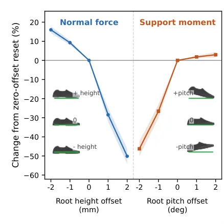
Figure 1: Contact sensitivity to small root-pose errors. Millimeter-scale height and degree-scale pitch changes strongly affect the simulated support wrench.
The three-stage learning system
The method has three explicitly separated stages. First, it relabels hardware windows with contact state, base velocity, and simulator-side stance pose. Second, it trains the UAN by replaying those labeled windows. Third, it freezes the UAN and trains a task policy in the augmented simulator. The deployed artifact is only the task policy.
flowchart LR
    A["Multi-frame proprioception
joint states and prior targets"] --> B["Six state estimators
velocity, contact, foot pose"]
    B --> C{"Contact probability
at least 0.8"}
    C -- "No" --> D["Discard replay window"]
    C -- "Yes" --> E["Contact-weighted fusion
root height and gravity"]
    E --> F["Contact-consistent hardware replay"]
    F --> G["PPO trains UAN
joint-target residual"]
    G --> H["Freeze UAN
inside nominal simulator"]
    H --> I["PPO trains task policy"]
    I --> J["Deploy task policy only"]
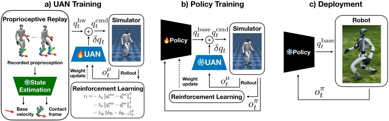
Figure 2: The original pipeline. The UAN is learned through replay, frozen during task learning, and omitted from the hardware deployment path.
Formal objective: correct the input, not the state
Let $s_t$ be the robot state, $a_t$ the action, $f(s_t,a_t)$ the hardware transition, and $f_{\mathrm{sim}}(s_t,a_t)$ the nominal simulator transition. A state-correction model would overwrite the simulator output directly. Contact-UAN instead learns a residual $\mu$ on the simulator input:
$$\min_{\mu}\mathbb{E}_{(s_t,a_t)}\left[\left\|f(s_t,a_t)-f_{\mathrm{sim}}\bigl(s_t,a_t+\mu(o_t^\mu)\bigr)\right\|_2^2\right].$$
Because the simulator still computes contact and integration, the network cannot invent an arbitrary next state. It can only shift the command presented to the existing actuator and contact models. This restriction is a structural defense against reward hacking by an unconstrained dynamics model.
For the Unitree G1 implementation, the residual acts on joint-position targets:
$$q_t^{cmd}=q_t^{base}+\delta q_t,\qquad \delta q_t=\mu(o_t^\mu).$$
During UAN training, $q_t^{base}=q_t^{hw}$, the target recorded on hardware. During downstream policy training, the same slot receives the task policy output. Deployment needs no extra network because only the task policy is exported.
Estimating a simulator-side contact state from proprioception
The state-estimation module predicts six quantities from a short history of onboard measurements: base linear velocity, two foot-contact probabilities, two stance-foot heights, and two stance-foot projected-gravity vectors. The input contains IMU angular velocity, projected gravity, joint positions, joint velocities, and previous targets. No external motion capture is used.
A crucial choice is to train foot-height and foot-orientation regressors only on stance samples. Swing feet travel over a much larger range, so an all-phase regression can reduce mean squared error by fitting gait phase while missing the small load-dependent variation that controls contact force. The contact classifier first separates stance from swing; the pose regressors then learn within the physically relevant subset.
Contact predictions are fused rather than converted into a hard left-or-right decision. With foot index $i\in\{L,R\}$, probability $\hat p_{i,t}$, and threshold $p_{th}$, the weights are:
$$w_{i,t}=\hat p_{i,t}\mathbf{1}[\hat p_{i,t}\ge p_{th}],\qquad \alpha_{i,t}=\frac{w_{i,t}}{\sum_j w_{j,t}+\varepsilon}.$$
The paper uses $p_{th}=0.8$. A window with no confident contact is discarded, because no stance foot exists from which to recover a root pose that can reproduce a support wrench.
For each confident foot, forward kinematics converts the estimated foot height into a root-height candidate. If $\hat h_{i,t}$ is the estimated foot height above the terrain and $h^{fk}_{i,t}(z=0)$ is the foot height obtained with zero root height, the fused root height is:
$$\hat z_t^{(i)}=\hat h_{i,t}-h^{fk}_{i,t}(z=0),\qquad \hat z_t=\sum_i\alpha_{i,t}\hat z_t^{(i)}.$$
Orientation uses the same contact weights. A foot-frame projected-gravity prediction is rotated into the root frame with forward kinematics, then the candidates are normalized and averaged:
$$\hat g_t^{(i)}=\operatorname{normalize}\left(R_{R\leftarrow F_i}(q_t)\hat g_{i,t}^{F_i}\right),\qquad \hat g_t=\operatorname{normalize}\left(\sum_i\alpha_{i,t}\hat g_t^{(i)}\right).$$
On flat terrain, this projected-gravity vector determines root roll and pitch in the yaw-invariant local frame. Combined with root height and base velocity, it completes the reset state used by replay. The estimator is trained only in simulation; its hardware transfer depends on load-dependent proprioception remaining informative across the actuator gap.
| Estimator | Output | Replay use | Architecture and loss |
|---|---|---|---|
| Base velocity | Three linear velocities | Complete the floating-base initial state | 256-256-256 MLP, MSE |
| Contact status | Left and right probabilities | Reject windows without confident support | 128-128 MLP, BCE-logits |
| Stance-foot height | One height per foot | Generate root-height candidates by FK | Stance-only 256-256-256 MLP, MSE |
| Stance-foot orientation | Projected gravity per foot | Generate root roll and pitch candidates | Stance-only 256-256-256 MLP, MSE |
| Fusion | Root height and projected gravity | Weight candidates by contact probability | Three-frame history, threshold 0.8 |
The UAN sees only local actuator history
The residual network receives a three-frame history of target-position error and joint velocity:
$$o_t^\mu=\left[(q^{base}-q)_{t-H_\mu+1:t},\dot q_{t-H_\mu+1:t}\right],\qquad H_\mu=3.$$
At a 50 Hz policy rate, three frames span about 60 ms. The observation is intentionally small: it excludes whole-body pose, contact labels, and future commands. This prevents the residual from memorizing task context and biases it toward a reusable actuator response.
G1 has 29 controlled joints belonging to five actuator families. The UAN uses one $6-128-128-1$ ELU network per family and shares that network across joints of the same hardware type. The resulting 174-dimensional observation is reshaped by joint and processed with family-specific einsum weights. This parameter sharing is an architectural statement about what should transfer: actuator behavior, not a particular gait.
Instead of fitting the residual with trajectory regression, the paper optimizes it through PPO in a replay environment. Each episode samples one labeled hardware window, primes three history steps, and rolls out 24 recorded targets over 480 ms. There are 4096 parallel environments, the residual is clipped to $\pm1.0\,\mathrm{rad}$, and only windows satisfying the contact threshold are valid.
The replay reward is:
$$r_t=-1000\left\|\bar q_t^{sim}-\bar q_t^{hw}\right\|_2^2-0.1\left\|\bar{\dot q}_t^{sim}-\bar{\dot q}_t^{hw}\right\|_2^2-0.01\left\|\delta q_t-\delta q_{t-1}\right\|_2^2.$$
The residual-magnitude regularizer has weight zero, while residual-rate regularization has a small negative weight. The authors do not ask the correction to be sparse. They ask it to remain smooth. This allows a persistent blind spot in the nominal actuator model to be compensated, while suppressing high-frequency residuals that would be destructive for both policy learning and hardware.
Freezing the model is part of the method
After replay learning, the UAN parameters are frozen. Every downstream policy action is passed through the same deterministic residual before the simulator applies its PD controller, actuator envelope, and contact solver. The task reward updates only the policy, so the learned actuator correction cannot drift toward whichever behavior the policy happens to explore.
The augmented simulator also removes some robot-specific randomization used by the baseline. Joint encoder bias and torso center-of-mass offsets can be dropped because the residual now models the actual hardware more directly. Ground friction and external pushes remain randomized because they describe the environment rather than a known actuator defect.
Running and jumping use a torque-speed envelope. Let $\bar\tau_j$ be stall torque, $\bar{\dot q}_j$ be no-load speed, and $r_j=\dot q_j/\bar{\dot q}_j$. The admissible torque interval is:
$$-\bar\tau_j\left[1+\max(\min(r_j,0),-1)\right]\le\tau_j\le\bar\tau_j\left[1-\max(\min(r_j,1),0)\right].$$
This envelope is asymmetric: braking torque remains available while torque in the direction of motion decreases with speed. The nominal target is clipped before the residual is added in simulation, and the same clipping is used during hardware deployment.
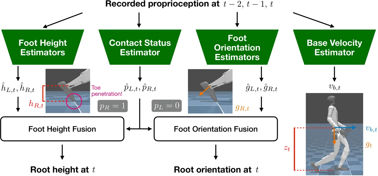
Figure 3: Contact-gated foot-pose estimation and forward-kinematic fusion recover the root pose required for hardware replay.
How the released code matches the paper
The first correspondence is src/mjlab/rl/uan_actor.py. Its module docstring describes five shared $6-128-128-1$ ELU actuator networks, each using three frames of target-position error and joint velocity. The constructor rejects any configuration other than 29 joints, five families, three history frames, two observation blocks, 128-unit hidden layers, ELU activations, and no observation normalization. _per_joint_forward selects weights with joint_to_actuator and applies the family network through an einsum over batch, joint, and input dimensions.
The second correspondence is src/mjlab/tasks/uan/mdp/actions.py. ReplayResidualJointPositionAction.process_actions scales and clips the raw residual, obtains the current recorded target from ReplayWindowCommand, and stores current_target + residual. apply_actions writes that sum as the simulated joint-position target. This is the exact command-channel behavior represented by the paper's objective.
The replay configuration supplies a third concrete link. src/mjlab/tasks/uan/mdp/replay_command.py sets history_horizon=3, require_contact_at_reset=True, and contact_threshold=0.8. The action config clips residuals at 1.0 rad, and rewards.py implements position MSE, velocity MSE, residual L2, and residual-rate L2 as separate terms. These files turn the paper description into executable constraints rather than leaving it as a conceptual block diagram.
| Item | Value | Reason |
|---|---|---|
| Robot model | Unitree G1, 29 joints, five actuator families | Share dynamics knowledge by hardware type |
| UAN input | Two blocks, three frames, 174 dimensions | Local error and velocity over roughly 60 ms |
| Family network | 128-128-1, ELU, biases enabled | Model load-dependent actuator nonlinearity |
| Replay batch and horizon | 4096 environments, 24 steps, 480 ms | Cover short contact and actuator transients |
| Residual range | $\pm1.0\,\mathrm{rad}$ | Avoid implausible early corrections |
| Valid reset | At least one foot with contact probability 0.8 | Guarantee a definable support state |
| Timing | 200 Hz physics, decimation 4, 50 Hz policy | Let the simulator integrate contact accurately |
Evidence: initialization and actuator error are separated
The controlled sim-to-sim study first checks whether contact-conditioned estimation actually recovers useful foot penetration. A direct pose regressor trained across all gait phases has much larger contact-height RMSE because swing-foot variation dominates. Restricting pose learning to stance samples reduces that error by roughly an order of magnitude, even in a hard target simulator with unseen actuator perturbations.
The reset ablation then links estimation quality to policy transfer. With a direct-estimator reset, retrained policies survive 20 seconds only 49.8% of the time in the target simulator. The contact-consistent estimated reset reaches 96.7%; oracle variants range from 96.6% to 98.4%. This is the strongest evidence that the simulator reset, not just the regression loss, controls what the residual learns.
A second experiment asks whether the UAN merely compensates for remaining reset error. With estimated initialization, adding the residual reduces 24-step joint-position RMSE from 0.0750 to 0.0239 rad. With ground-truth initialization, it still reduces RMSE from 0.0720 to 0.0184 rad. The improvement persists when initialization is exact, so actuator discrepancy has an independent contribution.
On held-out hardware running data, the paper replays identical recorded targets from identical relabeled states in the nominal and UAN-augmented simulators. The aggregate commanded-torque usage mismatch falls by 69.2%. Since commands and initial states match, the remaining difference is attributed to actuator modeling in a contact-rich motion rather than a changed task or trajectory.
| Condition | Metric | Result | Interpretation |
|---|---|---|---|
| Direct-estimator reset | 20-second survival | 49.8% | Incorrect contact state contaminates residual learning |
| Contact-consistent estimate | 20-second survival | 96.7% | Onboard sensing approaches oracle transfer |
| Component or full oracle | 20-second survival | 96.6% to 98.4% | Estimation is no longer the dominant bottleneck |
| Estimated state, no / yes UAN | 24-step joint-position RMSE | 0.0750 / 0.0239 rad | Residual corrects real transition error |
| Ground-truth state, no / yes UAN | 24-step joint-position RMSE | 0.0720 / 0.0184 rad | Benefit survives exact initialization |
| Held-out running replay | Aggregate torque mismatch | 69.2% lower | Contact-rich torque usage aligns more closely |
Hardware transfer beyond qualitative motion
The hardware UAN is trained from 6.5 minutes of real walking. The data-collection policy varies gait frequency and swing height so that it records different stance durations, swing speeds, and impacts. The same residual is then reused for tasks that were not represented by large target-specific hardware datasets.
Running is evaluated at commanded speeds of 1.0, 2.0, and 2.5 m/s over a fixed 30-foot course, with five trials per policy and speed. The UAN policy tracks velocity while reducing torque use by about 20%. At 3.0 m/s, the baseline overheats and enters safe damping after a few seconds, whereas the UAN policy achieves $3.13\pm0.06\,\mathrm{m/s}$.
Force tracking connects the end effector to a dynamometer through an exercise band, which forces the robot to coordinate its legs and torso rather than move only an arm. Across four hardware trials per commanded force, the UAN policy reduces average tracking error by $42.8\pm12.1\%$, with the largest gains under high load. At zero command it can also yield compliantly when pulled.
Combining that force policy with a proprioceptive end-effector estimator and PD outer loop produces closed-loop circular impedance tracking using onboard sensing. For jumping, both baseline and UAN policies track a reference before task-reward fine-tuning. The UAN version jumps higher; after fine-tuning, the no-UAN policy fails on landing while the UAN policy lands stably and withstands pushes. The UAN used here still comes from walking data.
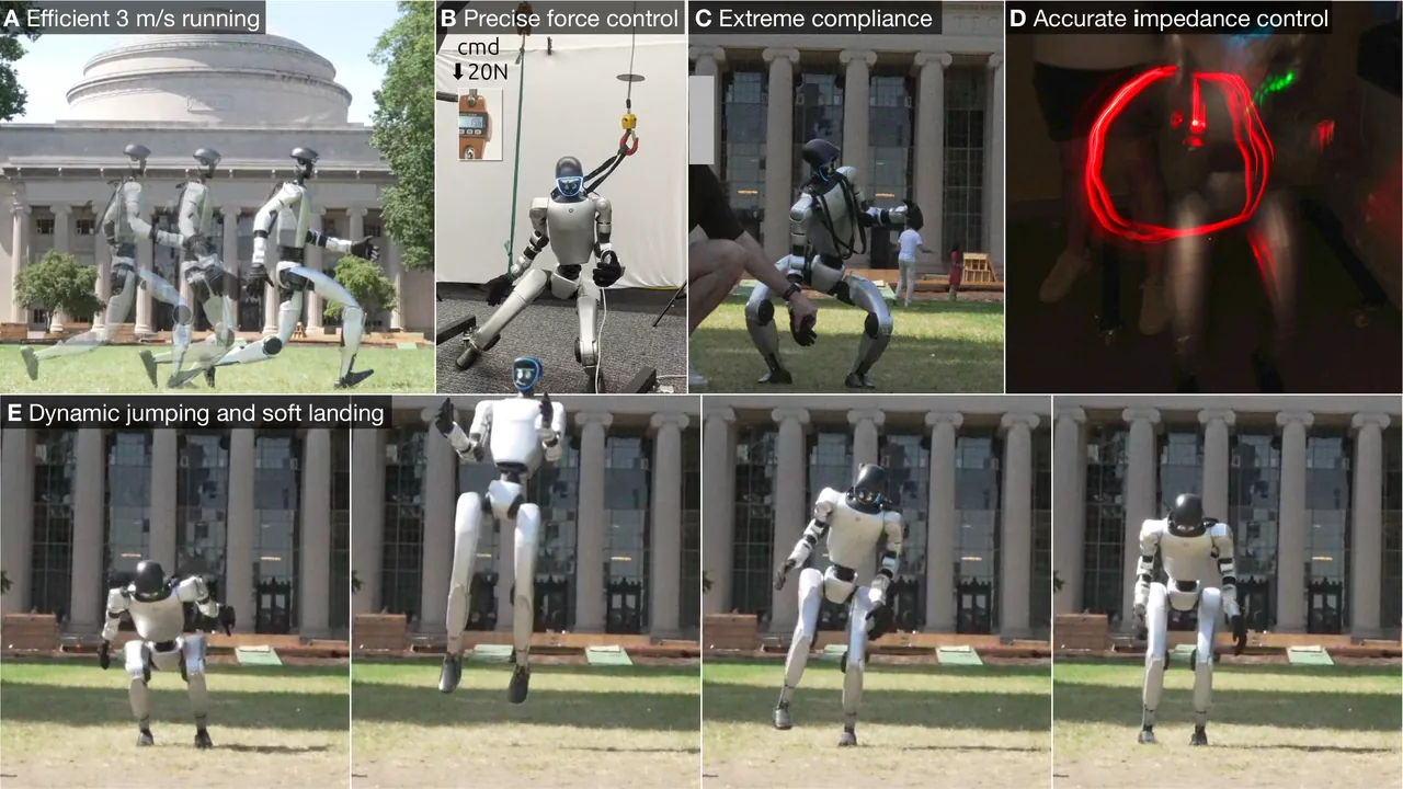
Figure 4: Five hardware behaviors whose success depends on torque, load, and impulse fidelity rather than motion appearance alone.
| Test | Comparison | Result |
|---|---|---|
| Running efficiency | Baseline versus UAN | About 20% lower torque usage at comparable speed |
| 3.0 m/s running | Baseline versus UAN | Baseline reaches thermal safe damping; UAN achieves 3.13 ± 0.06 m/s |
| End-effector force | Baseline versus UAN | Average tracking error reduced by 42.8 ± 12.1% |
| Position residual | Replay, survival, XY, yaw, power | 0.00349 rad; 97.34%; 0.391 m/s; 0.185 rad/s; 69.29 W |
| Torque residual | Replay, survival, XY, yaw, power | 0.00571 rad; 98.17%; 0.387 m/s; 0.214 rad/s; 69.25 W |
| Supervised torque | Replay, survival, XY, yaw, power | 0.00565 rad; 97.56%; 0.394 m/s; 0.215 rad/s; 71.90 W |
Data efficiency and alternatives
The controlled world-model comparison is striking. In the target simulator, UAN reaches 100% normalized episode length with 5 minutes of target data. A best-effort G1 adaptation of an offline fully learned world model uses about 33 hours, roughly 400 times more. Training a policy from scratch in that model reaches 6.8%, fine-tuning reaches 38.2%, and the nominal baseline is 32.6%.
This does not show that fully learned world models are inherently weak. Their job is much broader: they must reproduce every component needed for imagined rollouts. UAN inherits most of the simulator and spends its data on one narrow source of error. The sample-efficiency gap reflects that structural choice.
A matched comparison also tests position residuals, torque residuals, and a torque-supervised actuator model. The position residual gives the best replay fit, while all three reach similar downstream survival, velocity, yaw, and power. Position residuals are attractive because they avoid torque labels and preserve the position-control deployment interface.
Robustness experiments corrupt training data with 0.5°, 1°, and 2° IMU pitch biases or causal velocity filtering at 20, 10, and 5 Hz. Reported 20-second survival stays between 97.1% and 100%; joint-position and velocity replay RMSE remain within 8% and 11% of clean results, and command-tracking error within about 15%. These are structured perturbations, not evidence that arbitrary sensing failures are safe.
The jumping reward uses a ballistic estimate to convert takeoff vertical velocity into a desired peak height:
$$h_{\mathrm{ballistic}}=\frac{\max(v^{takeoff}_{COM,z},0)^2}{2g}.$$
This reward specifies the task, while the UAN changes how believable the simulator's torque and impact response is during optimization. The distinction matters: a higher reward is not useful if the policy reaches it through an actuator response the hardware cannot reproduce.
Limitations
The authors explicitly state that the current UAN does not model coupled actuator effects. Each network acts on one joint within its actuator family, which is parameter-efficient but cannot represent how loading or velocity at one joint changes another joint's transmission response. A whole-body model or cross-joint attention could address this.
The authors also note that motor-temperature effects are absent. Temperature evolves slowly relative to the control loop and short data windows, so it is difficult to identify from 6.5 minutes of proprioception. Covering it would require heat modeling, longer observations, or additional sensors.
There are further boundaries in the method as evaluated. The state estimators assume flat terrain and use a yaw-invariant local frame, while the hardware demonstrations are primarily on flat ground. Stairs and uneven contact geometry would make both foot-pose supervision and reset reconstruction substantially harder.
The residual's observation horizon is three policy steps. That is a sensible local actuator memory, but it cannot identify wear, temperature, or long-term changes in payload. The $\pm1.0\,\mathrm{rad}$ residual clip likewise protects training rather than promising recovery from severe mechanical faults.
Finally, the released code supports reproduction but does not package the hardware dataset or pretrained policies. The paper's 6.5-minute result is data-efficient, yet it still depends on a specific G1 platform, contact model, calibration, and deployment stack. Cross-robot transfer would require new hardware trajectories and relabeling.
Conclusion
Contact-UAN makes a precise architectural argument: learn only where the analytical simulator is least reliable and the downstream task is most sensitive. The actuator command channel is narrow enough to preserve contact physics and integration, while expressive enough to capture nonlinear friction, saturation, and load response that alter force generation.
The prerequisite is equally important. Contact-rich replay must begin from a state that produces hardware-consistent support forces. Without that step, a residual model has no way to distinguish a genuine actuator gap from a reset artifact. The 49.8% to 96.7% survival jump shows that this data-engineering decision changes whether transfer works, not merely how well a regression fits.
The resulting system demonstrates a practical tradeoff between analytical simulation and learned dynamics. It retains the simulator's generalization structure and adds hardware evidence through a small residual, achieving efficient running, accurate force control, compliant interaction, and robust jumping from 6.5 minutes of walking data. The next technical step is to extend the model to coupled and slow thermal effects without surrendering the physical prior that makes the current result data-efficient.
Golden line: The decisive sim-to-real gap is often not whether a motion looks right, but whether the ground feels the same force at the same instant.
Source note. This analysis is based on the full arXiv:2610.18991v1 paper, its official project page, and public code at commit 55de136. Reported numbers come from the paper's main text, Figures 5 through 8, Appendix Table 15, and the released implementation.