PAPER DEEP DIVE
What Visual Representations Do World Action Models Need?
World Action Models inherit their visual foundation from video-generation VAEs trained for pixel reconstruction, which leaves manipulation-relevant information underrepresented. This study holds one Wan2.2 dual-expert backbone and one training protocol fixed and compares 13 frozen visual representations, 5 feature-integration mechanisms and multiple feature compositions on LIBERO-Plus. Three findings emerge. First, general-purpose representations beat specialized ones on average (82.2 vs 80.0 overall success), and every perturbation family is topped by a general source. Second, channel-wise joint prediction is the strongest mechanism (81.5 mean over 13 sources, 5.1 points ahead of the runner-up), and its gain comes mainly from predicting future features rather than from conditioning on the current frame. Third, extra sources help only when complementary: the largest additional gain is 3.7 points, and pairing a distilled encoder with its own teacher (C-RADIOv4 + DINOv3) drops success to 78.6. The resulting recipe R²-WAM (DINOv3 + UniTok + V-JEPA 2.1, channel-wise) reaches 84.7% on RoboCasa GR1 Tabletop (+5.9) and 92.8% on RoboTwin 2.0 (+2.2), and improves all four Galbot G1 real-robot tasks by roughly 10 points.
One-sentence summary
This paper proposes no new representation. Instead it holds one world action model backbone and one training protocol fixed, and runs controlled comparisons over 13 pretrained visual representations, 5 feature-integration mechanisms, and multiple feature compositions. Three actionable conclusions come out: default to a general-purpose representation, default to channel-wise joint prediction, and add extra representation sources only when they are genuinely complementary. Instantiating those three rules as R²-WAM yields 84.7% success on RoboCasa GR1 Tabletop and 92.8% on RoboTwin 2.0.
1. Background and Motivation
World Action Models (WAMs) repurpose pretrained video generation models as robot controllers. A video expert predicts future video latents, an action expert predicts action chunks, and the two are coupled through joint attention. Work such as DreamZero, LingBot-VA and Fast-WAM has established that the visual structure and temporal dynamics priors carried by video pretraining do transfer to control. What that line of work inherits, almost without comment, is the variational autoencoder (VAE) latent space of the video model.
The VAE is trained for pixel reconstruction. Reconstruction forces the latent to keep information about what the scene looks like; it does not force the latent to keep information about how to act on the scene. Object semantics, spatial relations, contact and affordance extent are not explicitly prioritized by a reconstruction objective. The result is a structural mismatch: the visual foundation of a WAM is optimized for seeing, while its job is doing.
Several recent efforts try to close that gap with external visual representations — some through representation alignment, some through action conditioning, some through joint prediction — and all report gains in performance and robustness. The trouble is that each of them picks a representation from a prior belief about which visual capability a WAM is missing, and then couples that choice to a bespoke integration mechanism. A reader cannot tell whether the gain comes from the representation itself or from the injection scheme designed around it.
The second unanswered question is composition. Manipulation asks for many things from vision at once — semantics, geometry, object extent, motion, interaction — which hints that several representations may be needed. Yet additional sources can also inject redundant information, or interfere with one another during optimization. Whether multi-source composition is monotonically beneficial is an empirical question that only experiments can settle.
This paper starts by decoupling those two variables. Under a shared WAM backbone and a shared training protocol, the authors run controlled comparisons over representation source, integration mechanism, and feature composition, and pose three research questions: RQ1, which visual representations improve WAM performance; RQ2, which integration mechanism benefits most from external features; RQ3, whether composing more representation sources keeps paying off. In the paper's own words: "Systematic comparisons across representation types remain limited, leaving unclear which visual representations best support robot manipulation in WAMs."
2. Preliminaries
Flow matching. Every generative quantity in this paper — video latents, actions, external features — is trained with flow matching. Given a clean sample $x_0$ and noise $\epsilon$, the interpolation $x_\tau=(1-\tau)x_0+\tau\epsilon$ is formed, the model regresses the velocity field $v=\epsilon-x_0$, and the loss is mean squared error on that velocity. At inference the state starts from pure noise and is denoised step by step under a scheduler. Once this is clear, every mention of "joint denoising" or "future feature prediction" in the paper simply means: treat the external feature as one more generative quantity with the same shape as the video latent.
The dual-expert WAM backbone. The base model consists of a video expert initialized from the Wan 2.2 video generation model and a separate action expert. They interact through joint attention with an asymmetric mask: action tokens may attend to both video and action tokens, while video tokens attend only to video tokens. Both experts read the T5-encoded language instruction through cross-attention and are additionally conditioned on robot state and flow time $\tau$. The direction of that mask matters, because it decides what the action expert is allowed to see — and it is exactly where the five integration mechanisms below do their work.
LIBERO and LIBERO-Plus. LIBERO is a simulation benchmark of 40 tabletop manipulation tasks, evaluated here with 50 rollouts per task following the Fast-WAM protocol. The authors found performance on LIBERO close to saturated, so they take the same checkpoints zero-shot to LIBERO-Plus (LP): seven perturbation families (camera viewpoint, robot embodiment, language, lighting, background, image noise, layout), with 10,030 episodes per evaluation seed. LP therefore carries most of the discriminative power in this paper.
3. Study Design: One Backbone, Three Questions
3.1 Base training objective and notation
The base WAM predicts future video latents $z_{1:T}^{\mathrm{vae}}$ and the action chunk $a$ simultaneously, and is trained on a weighted sum of the two flow-matching losses:
$$\mathcal{L}_{\mathrm{WAM}}=\mathcal{L}_{\mathrm{FM}}(z_{1:T}^{\mathrm{vae}})+\lambda_{\mathrm{act}}\mathcal{L}_{\mathrm{FM}}(a) \tag{1}$$
Here $\mathcal{L}_{\mathrm{FM}}$ is the mean squared error between predicted and target velocity for each modality, and $\lambda_{\mathrm{act}}$ is the action loss weight (1.0 in the experiments). Notation: $t=0$ denotes the current observation, $t=1,\ldots,T$ the future sequence, and $\tau$ the flow time; so $z_0^{\mathrm{vae}}$ is the current-frame VAE latent and $z_{1:T,\tau}^{\mathrm{vae}}$ is the future video latent at flow time $\tau$. At inference both the future video and the action are initialized from noise and denoised jointly.
3.2 Thirteen representations and the general / specialized split
The authors compare 13 pretrained visual encoders. All are frozen, all extract features only from the RGB observations visible to the base WAM, and all are grouped by pretraining objective into six emphases: visual self-supervision (VC-1, VideoMAE V2, V-JEPA 2.1, DINOv3, LingBot-Vision), language association (SigLIP 2, Qwen3.5), segmentation supervision (SAM 3), geometry supervision (VGGT-Ω), interaction-oriented pretraining (HRP, DynaFLIP), and multi-objective or multi-teacher distillation (UniTok, C-RADIOv4). On top of that sits one decisive dichotomy: encoders pretrained for broad visual or vision-language transfer are labeled general-purpose, while encoders pretrained mainly for one specific visual capability are labeled specialized. The split is not drawn by accuracy but by pretraining intent — which is precisely why it shapes the form of the RQ1 conclusion.
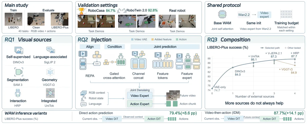
Figure 1 (paper Figure 1): study overview. Under a shared training protocol the paper compares visual feature sources (RQ1), five integration mechanisms (RQ2) and feature composition (RQ3) side by side, then validates across backbones and on a real robot.
3.3 The five integration mechanisms
Write the current and future external features as $f_0$ and $f_{1:T}$ (superscript $k$ marks the source when needed), and the future feature state at flow time $\tau$ as $f_{1:T,\tau}$. The five mechanisms cover three families of ideas: representation alignment, action conditioning, and joint prediction.
Representation alignment (REPA). A trainable projector maps an intermediate hidden state of the WAM into the external feature space and aligns it, under a cosine-distance loss, with the spatially corresponding features of a frozen teacher. Alignment is applied to the output of the 8th block of the video expert, the projector is a three-layer MLP, and the teacher trajectory is spatially resampled onto the video token grid — the observation slice is kept while the eight future slices are averaged into two groups. Its loss is:
$$\mathcal{L}_{\mathrm{REPA}}=1-\frac{1}{|\Omega|}\sum_{i\in\Omega}\left\langle\widehat{P(h_i^{8})},\widehat{f_i}\right\rangle \tag{3}$$
where $\Omega$ is the set of valid future tokens (excluding the observation slice) and the wide hat denotes $\ell_2$ normalization. The frozen teacher and the projector exist only during training; at inference the whole alignment branch is removed. That is the most fundamental difference between REPA and the other four mechanisms.
Gated cross-attention. One feature cross-attention path is inserted into each of the 30 blocks of the action expert: the query is the normalized action state after mixed attention, the key and value come from the current observation feature $f_0$ passed through an adapter projection. The output is scaled by a learnable scalar gate $\tanh(g_\ell)$ before being added back to the residual, and $g_\ell$ is initialized at 0 so the new branch starts perfectly neutral:
$$\widetilde{h}_a^{\ell}=\bar{h}_a^{\ell}+\mathrm{CA}_{\mathrm{text}}^{\ell}(\bar{h}_a^{\ell},c)+\tanh(g_\ell)\,\mathrm{CA}_{\mathrm{feat}}^{\ell}(\bar{h}_a^{\ell},f_0) \tag{4}$$
This mechanism predicts no future features and carries no auxiliary loss; the frozen encoder and the cross-attention branch remain active at inference. For REPA and the three joint-prediction mechanisms, the total objective is written uniformly as:
$$\mathcal{L}=\mathcal{L}_{\mathrm{WAM}}+\lambda_{\mathrm{aux}}\mathcal{L}_{\mathrm{aux}} \tag{2}$$
where $\mathcal{L}_{\mathrm{aux}}$ is the cosine alignment loss for REPA and the future-feature flow-matching loss for the joint-prediction mechanisms, while gated cross-attention trains on $\mathcal{L}_{\mathrm{WAM}}$ alone. The default auxiliary weight is 1.0, and 0.1 for the feature expert and for REPA.
Channel-wise concatenation. The external feature is spatially aligned to the VAE latent grid and concatenated along the channel dimension; the input and output projections of the video expert are widened accordingly, so the expert jointly predicts two velocity fields — the VAE latent and the external feature — while the layout of video tokens and the attention mask stay completely unchanged. Observation features are kept clean, future VAE latents and future features are noised together and predicted together. At inference the future feature is initialized from noise and takes part in joint denoising, but only the VAE latent is decoded in the end.
Token-wise concatenation and the feature expert. Token-wise concatenation flattens the external feature into its own token sequence $[V_0,V_{1:T},F_0,F_{1:T},A]$, maps it to the video expert's hidden width through a separate input projection, shares all Transformer blocks with the VAE tokens, and adds a prediction head that maps back to the source dimension $C_f$; the velocity target for the feature stream is $\epsilon_f-f_{1:T}$. The feature expert replaces sharing with separation: an independent 30-block Transformer with hidden width 1024, FFN width 4096 and 24 heads, which exchanges information with the video and action experts through masked joint attention while keeping its own projection and feed-forward parameters. All three belong to joint prediction; they differ exactly in where fusion happens and whether parameters are shared.
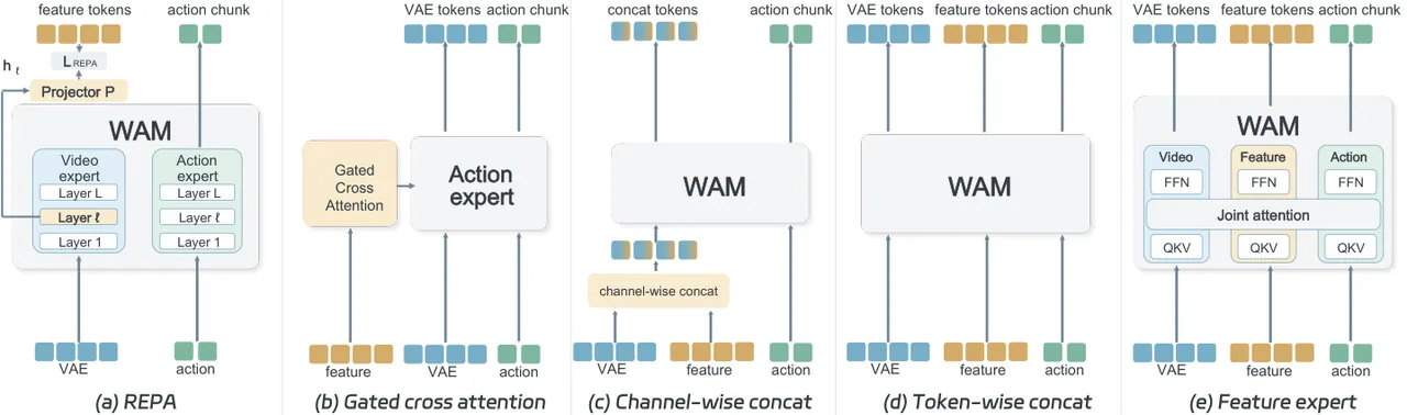
Figure 2 (paper Figure 2): structural comparison of the five integration mechanisms. (a) REPA hidden-state alignment; (b) gated cross-attention; (c) channel-wise concatenation; (d) token-wise concatenation; (e) feature expert.
3.4 The composition protocol
Composition experiments fix channel-wise concatenation as the common mechanism. For a source set $\mathcal{K}$, per-source features are concatenated along the channel dimension in a fixed order, and the current and future frames are merged into the widened latent separately:
$$f_t=\mathrm{Concat}_{\mathrm{ch}}\{f_t^k: k\in\mathcal{K}\},\quad \widetilde{z}_0=[z_0^{\mathrm{vae}},\,f_0]_{\mathrm{ch}},\quad \widetilde{z}_{1:T,\tau}=[z_{1:T,\tau}^{\mathrm{vae}},\,f_{1:T,\tau}]_{\mathrm{ch}} \tag{8}$$
The current state $\widetilde{z}_0$ stays clean, each source contributes its own future-feature loss, and the total auxiliary loss is the sum over sources:
$$\mathcal{L}_{\mathrm{aux}}=\sum_{k\in\mathcal{K}}\mathcal{L}_{\mathrm{FM}}(f_{1:T}^k) \tag{9}$$
Source-specific preprocessing and concatenation order are identical between training and evaluation. This protocol turns composition into a purely additive experiment: each extra source adds one channel group and one prediction loss, and nothing else changes.
3.5 Why a mechanism works: prediction ablation and action sensitivity
To explain the advantage of channel-wise concatenation the authors run two diagnostics. The first is a prediction ablation, separating "current-feature conditioning" from "future-feature prediction" inside channel-wise concatenation. The second is local action sensitivity: writing the final normalized action chunk as $A_m(F;\xi)\in\mathbb{R}^{32\times 7}$ (where $F$ is the raw current-frame DINOv3 feature and $\xi$ collects all other fixed inputs and the realized sampling noise), they differentiate through the full ten-step denoising process to obtain the action-feature Jacobian block:
$$J_{g,c,p}=\frac{\partial a_g}{\partial F_{c,p}} \tag{5}$$
where $a_g$ is one of the translation, rotation or gripper action groups (dimensions 96, 96 and 32), and $F_{c,p}$ is the full channel set of one $2\times 2$ feature patch inside a $7\times 7$ diagnostic grid on a given camera. To avoid materializing the full Jacobian, a Rademacher random projection $z_r$ estimates the vector-Jacobian product and gives a local sensitivity:
$$\widehat{s}_{g,c,p}=\left[\frac{1}{R}\sum_{r=1}^{R}\left\|\frac{\partial (z_r^{\top} a_g)}{\partial F_{c,p}}\right\|_2^2\right]^{1/2} \tag{6}$$
Averaging over the 49 grid cells and the two camera views yields the sensitivity scalar for mechanism $m$ and action group $g$ under observation state $o$:
$$\widehat{S}_{m,g}(o)=\frac{1}{2\cdot 49}\sum_{c=1}^{2}\sum_{p=1}^{49}\widehat{s}_{m,g,c,p}(o) \tag{7}$$
The point of this diagnostic is that it does not compare success rates. It measures directly how strongly action generation locally depends on the external visual input. REPA is not applicable here because no external feature reaches it at inference — which is itself evidence that its information pathway belongs to training time.
flowchart TB
    subgraph SRC["13 frozen encoders, 6 pretraining emphases"]
        D[DINOv3]
        U[UniTok]
        V[V-JEPA 2.1]
        O[SAM 3 / VGGT-Omega / HRP / SigLIP 2 / ...]
    end
    subgraph MECH["5 integration mechanisms, shared WAM backbone"]
        R[REPA align]
        G[Gated cross-attn]
        C[Channel-wise concat]
        T[Token-wise concat]
        F[Feature expert]
    end
    WAM[Wan2.2 video expert + action expert]
    SRC --> MECH
    MECH --> WAM
    C -->|LP avg 81.5 pct, best| REC[R2-WAM recipe]
    D --> REC
    U --> REC
    V --> REC
    REC --> B1[RoboCasa GR1 Tabletop 84.7 pct]
    REC --> B2[RoboTwin 2.0 92.8 pct]
    REC --> B3[Galbot G1 real robot, 4 tasks]
Figure: the study-to-recipe chain of this paper. Thirteen frozen encoders enter one WAM backbone through five mechanisms; the winning channel-wise concatenation plus three complementary sources hardens into the R²-WAM recipe, which is then validated across backbones, benchmarks and a real robot.
4. Results and Interpretation
4.1 RQ1: a general-purpose representation is the default answer
All single-source experiments inject features with channel-wise concatenation, and the baseline is the VAE-only WAM. Overall success rates under the seven LP perturbation families (mean over three evaluation seeds) are:
| Representation source (group) | Camera | Background | Noise | Overall |
|---|---|---|---|---|
| VAE-only baseline | 51.2 | 62.0 | 66.6 | 74.7 |
| DINOv3 (general / self-supervised) | 64.2 | 83.9 | 86.0 | 84.0 |
| C-RADIOv4 (general / multi-teacher) | 62.6 | 86.2 | 86.6 | 83.5 |
| SigLIP 2 (general / language-associated) | 60.7 | 82.4 | 83.4 | 83.1 |
| V-JEPA 2.1 (general / self-supervised) | 63.0 | 80.7 | 84.4 | 82.4 |
| SAM 3 (specialized / segmentation) | 57.8 | 75.3 | 81.5 | 80.6 |
| VGGT-Ω (specialized / geometry) | 62.4 | 75.7 | 79.6 | 80.6 |
| HRP (specialized / interaction) | 52.6 | 82.2 | 81.2 | 79.8 |
Read the baseline first: the VAE-only WAM does well under language perturbation (91.1%) and lighting perturbation (94.3%), yet collapses under viewpoint change (51.2%), background change (62.0%) and image noise (66.6%). The robustness gap left by a reconstruction objective is not uniform. Now read the conclusion: general-purpose representations average 82.2% and specialized ones 80.0%, and in every one of the seven perturbation families the best mean comes from a general source — including viewpoint, background and noise, exactly the families one would expect a specialized capability to fix. HRP is trained on hand-object-contact supervision and should, by construction, understand manipulation best; under viewpoint perturbation it reaches only 52.6%, essentially level with the baseline. Takeaway 1 follows: do not pick a specialized encoder from a hypothesis about which capability is missing — default to a general-purpose representation.
The full per-source numbers behind the table are worth keeping in view, because they show the shape of the win rather than only its size. On the VAE-only baseline the seven families read 51.2 (camera), 77.8 (robot embodiment), 91.1 (language), 94.3 (lighting), 62.0 (background), 66.6 (noise) and 82.4 (layout), for an overall 74.7. DINOv3 lifts the overall to 84.0, and the lift is concentrated exactly where the baseline was weak. Across all 13 encoders the overall scores run DINOv3 84.0, C-RADIOv4 83.5, SigLIP 2 83.1, VC-1 82.5, LingBot-Vision 83.0, V-JEPA 2.1 82.4, UniTok 81.9, Qwen3.5 81.6, SAM 3 80.6, VGGT-Ω 80.6, HRP 79.8, DynaFLIP 78.8 and VideoMAE V2 77.5. Every one of them beats the baseline, which is the paper's quiet second message: adding almost any external representation helps; the interesting question is which one helps most and through which mechanism.
4.2 RQ2: where channel-wise joint prediction wins
In the full 13 representations × 5 mechanisms matrix, averaging the LP overall success rate across representations gives (aggregated here from the per-source data in the paper's Table 8):
| Integration mechanism | Mean LP overall across 13 sources | LP overall with DINOv3 | Feature pathway kept at inference |
|---|---|---|---|
| Channel-wise concatenation | 81.5 | 84.0 | Yes (joins the denoising) |
| Feature expert | 76.4 | 78.7 | Yes |
| REPA | 76.2 | 78.1 | No (training-time alignment) |
| Gated cross-attention | 74.7 | 73.9 | Yes (current-feature memory) |
| Token-wise concatenation | 72.7 | 76.1 | Yes |
Channel-wise concatenation leads the runner-up by 5.1 points at 81.5% on average, and the lead is not propped up by a few favorable sources: 12 of the 13 sources reach their own best score under channel-wise concatenation. The failures are more informative than the wins. Under token-wise concatenation V-JEPA 2.1 drops to 49.5% and SigLIP 2 to 66.4%, both below the VAE-only baseline — treating the feature as an independent token stream inside a shared Transformer is catastrophic for some feature geometries. Channel-wise concatenation has no source below 77.5% on the same set.
Why channel-wise? The prediction ablation gives the first layer of the answer. Inside DINOv3 plus channel-wise concatenation, keeping only future-feature prediction (dropping current-feature conditioning) reaches 81.9%, keeping only current-feature conditioning (predicting no future feature) reaches 76.5%, and having both reaches 84.0%. Most of the gain therefore comes from making the video expert learn to predict the future of the external feature; conditioning on the current frame is the smaller part. A shared-PCA visualization further shows that the future DINO features predicted by the video expert retain recognizable coarse spatial structure. The second layer comes from action sensitivity: channel-wise concatenation shows higher translation and rotation sensitivity than the other mechanisms in the approaching, grasping and placing states alike, meaning action generation really does use the added visual information more strongly. Both observations go into Takeaway 2: a new mechanism should support future-feature prediction and should let the action expert actually use the added features.
The mechanism means also expose a trap in how such comparisons are usually reported. Gated cross-attention averages 74.7% — numerically identical to the VAE-only baseline — and with DINOv3 it scores 73.9%, slightly below the baseline. A mechanism that keeps the frozen encoder active at inference, injects the current feature into all 30 action-expert blocks, and starts from a zero gate can still end up contributing nothing measurable. The paper's reading is that a current-feature memory alone is not what a WAM lacks; what it lacks is a target that forces the generative trunk to model the future of that feature.
4.3 RQ3: composition pays less, and pays conditionally
Starting from DINOv3 with channel-wise concatenation fixed, candidate sources are added one at a time. DINOv3 alone is worth +9.3 points (74.7 to 84.0), while the largest extra gain from any additional source across all evaluated compositions is only 3.7 points. The conditionality is finer still: SigLIP 2 adds +1.8 on top of DINOv3, but −0.4 once UniTok is already in the set, and only +0.2 when V-JEPA 2.1 is present as well. C-RADIOv4 is distilled from DINOv3, SigLIP 2 and SAM 3, and pairing it with DINOv3 pushes success down to 78.6% — teacher and student in the same set is double counting. Conversely V-JEPA 2.1 does add value on top of DINOv3 plus UniTok, consistent with its video-based predictive pretraining supplying complementary cues. Takeaway 3 is therefore: choose an additional source by how much task-relevant information it contributes beyond the representations already present, and treat composition as refinement rather than as the main lever.
4.4 Recipe validation: across backbones, benchmarks and a real robot
Hardening the three conclusions gives R²-WAM: DINOv3 plus UniTok plus V-JEPA 2.1, injected channel-wise. Adding HRP would buy another +0.4 (87.3 to 87.7), but the authors stop at three sources to keep the number of auxiliary encoders and prediction targets down. In the cross-backbone check, a direct action prediction backbone improves from 96.8 / 70.8 to 98.4 / 79.4 on LIBERO / LP, and a video-then-action (IDM) backbone from 98.6 / 73.6 to 99.1 / 87.7 — the recipe does not depend on the specific joint-denoising formulation. Cross-benchmark results:
| Benchmark | VAE-only | R²-WAM | Strongest comparators |
|---|---|---|---|
| RoboCasa GR1 Tabletop (24 tasks × 50 rollouts) | 78.8 | 84.7 (+5.9) | LAWA 80.8 / WALA 75.2 / DIAL 70.2 / FLARE 55.0 / DiT4DiT 50.8 / GR00T-N1.6 47.6 |
| RoboTwin 2.0 (50 tasks × 100 rollouts, clean+rand mean) | 90.6 | 92.8 (+2.2) | WALA-Wan 92.3 / LingBot-VA 92.2 / Fast-WAM 91.8 / InternVLA-A1 89.5 / StarVLA-α 88.3 / Motus 87.8 / π0.5 79.8 |
On the real robot, four tasks run on a Galbot G1 dual-arm platform with 20 trials per model per task: air-fryer meal preparation 50.0 to 60.0, instructed pick-and-place 70.0 to 80.0, cup pushing 65.0 to 75.0, and a sweeping task scored by debris collection rate 48.3 to 66.7. Each of the three binary tasks gains +10.0 points, and together they cover sequential manipulation and tool use, so the recipe's benefit crosses the simulation-to-reality boundary. The RoboCasa margin of +5.9 points is the more meaningful of the two benchmark numbers, since RoboTwin 2.0 is already near ceiling for this class of model at 90.6% baseline.
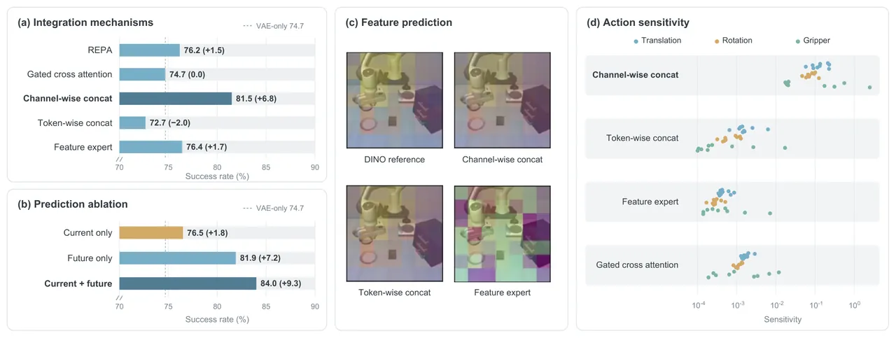
Figure 3 (paper Figure 3): mechanism analysis. (a) mean LP success of the five mechanisms across 13 sources; (b) the DINOv3 prediction ablation; (c) future-feature prediction visualized under shared PCA; (d) local action sensitivity scatter.
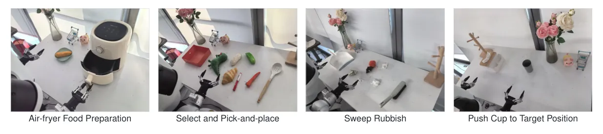
Figure 4 (paper Figure 5): the four real-robot scenes — air-fryer meal preparation, instructed pick-and-place, debris sweeping, and pushing a cup to a target position.
4.5 Implementation notes read from the author's feature-space repository
No official training code accompanies the paper, but the first author maintains a predecessor repository that trains in DINO and V-JEPA feature spaces on a Wan2.2 backbone. Three implementation details there line up with the paper's appendices and are the parts most likely to be gotten wrong when reimplementing channel-wise concatenation.
The first is feature extraction. The frozen encoder is loaded, switched to eval with gradients off, and only the patch tokens are kept: the CLS token and any register tokens are stripped by a prefix count read from the model config, after which the flat token sequence is folded back into a feature grid and resampled onto the target grid used by the video latent (wan/features/extractors.py:120-168).
# wan/features/extractors.py:120-168 (DINOv3FeatureExtractor, abridged)
self.model.eval().requires_grad_(False).to(config.device)
self.patch_size = int(getattr(self.model.config, "patch_size", 16))
self.num_prefix_tokens = 1 + int(getattr(self.model.config, "num_register_tokens", 0))

out = self.model(pixel_values=batch)
tokens = out.last_hidden_state
tokens = tokens[:, self.num_prefix_tokens:]        # drop CLS + register tokens
feature = _as_feature_grid(tokens, frames=..., height=..., width=...,
                           patch_size=self.patch_size, tubelet_size=1)
return resize_feature_grid(feature.float().cpu(), self.config.target_grid)
The second is the flow-matching target. The noisy input is built as $(1-\sigma)x_0+\sigma\epsilon$ and the regression target is the velocity $\epsilon-x_0$, exactly the convention assumed throughout the paper's losses (wan/features/modeling.py:229-240).
# wan/features/modeling.py:229-240 (flow_match_noisy_input, abridged)
"""Return noisy input and flow target for x_t=(1-sigma)x_0+sigma*eps."""
sigmas = sigmas.to(device=clean.device, dtype=clean.dtype).view(-1, 1, 1, 1, 1)
noisy = (1.0 - sigmas) * clean + sigmas * noise
target = noise - clean
return noisy, target
The third is the least obvious and the easiest to miss: high-dimensional DINO latents need a dimension-dependent timestep shift. With $\alpha=\sqrt{d_{\mathrm{eff}}/d_{\mathrm{base}}}$ and $d_{\mathrm{base}}=4096$, the flow time is remapped as $t'=\alpha t/(1+(\alpha-1)t)$, which moves sampling mass toward the noisier end for feature spaces wider than the VAE latent (wan/features/modeling.py:242-256). Feature preparation itself — the offline pass that writes per-episode feature tensors to disk before training — lives in scripts/feature_space/prepare_features.py:47-113.
# wan/features/modeling.py:242-256 (shifted_timestep, abridged)
"""Dimension-dependent timestep shift used for high-dimensional DINO latents."""
alpha = math.sqrt(float(effective_dim) / float(base_dim))   # base_dim = 4096
denominator = 1.0 + (alpha - 1.0) * t
return (alpha * t) / denominator.clamp_min(1e-12)
Training configuration reported in the paper is consistent with a standard large-scale setup: AdamW with learning rate 1e-4 decaying to 1e-6 on a cosine schedule, 5% warmup, weight decay 0.01, betas (0.9, 0.95), gradient clipping at 1.0, bf16 precision, an action horizon of 32 and 9 frames per view. LIBERO uses 40 tasks / 1712 demonstrations / 2 views / 224² inputs / action dimension 7 / batch 128 / 10 epochs; RoboCasa 24 tasks / 24000 demonstrations / 1 egocentric view / 224² / dimension 47 / batch 1024 / 5 epochs; RoboTwin 50 tasks / 27500 demonstrations / 3 views / 240×320 / dimension 14 / batch 1024 / 5 epochs.
5. Limitations
Stated by the authors. First, the composition route has limited marginal value: even the best evaluated composition gains less from its extra sources than the VAE-only baseline gains from its first strong general-purpose representation, so composition can only be a supplementary path. Second, to keep the number of auxiliary encoders and feature prediction targets manageable, the recipe stops at three sources — HRP's +0.4 is deliberately left on the table — and the larger composition space is unexplored.
Our reading. First, every comparison is one trained checkpoint per configuration with three evaluation seeds, so the reported uncertainty covers evaluation noise only, not training noise. A collapse like V-JEPA 2.1 at 49.5% under token-wise concatenation cannot be separated into "mechanism-level defect" versus "one unlucky optimization run", which means the confidence interval on the mechanism ranking is wider than the table suggests. Second, all 13 encoders are frozen and mostly at L scale; the study never touches encoder capacity, input resolution or whether fine-tuning is allowed — three knobs that could plausibly dominate the gains. The general / specialized dichotomy also rests on the authors' own reading of pretraining intent (C-RADIOv4, distilled from three teachers, is counted as general), and Takeaway 1 would be worded differently under another taxonomy. Third, discriminative power comes mainly from LIBERO-Plus, a single simulator family's perturbation benchmark, while real-robot validation is 4 tasks × 20 trials; behavior on longer horizons, mobile manipulation or tightly coupled bimanual tasks remains open.
6. Conclusion and Outlook
The contribution here is not a new model but a change of evidential standard: adding visual features to a WAM, previously driven by priors and taste, becomes a set of checkable controlled experiments. The resulting recipe is deliberately plain — put in one strong general-purpose representation, let it participate in joint prediction through channel-wise concatenation, then add sources only where complementarity is demonstrated. The gains R²-WAM shows on two mainstream manipulation benchmarks and on a real robot indicate that this plain route has not yet been beaten by more elaborate mechanisms. For follow-up work the paper points back at two places: stronger general-purpose visual foundation models, and integration mechanisms that let the action expert actually exploit visual information — the first sets the ceiling, the second decides how much of it is cashed in.
For practitioners the actionable residue is the implementation detail in Section 4.5: strip prefix tokens before folding features into a grid and resample to the latent grid, keep the velocity target as noise minus clean, and apply the dimension-dependent timestep shift when the feature space is much wider than the VAE latent. Those three choices are what make channel-wise joint prediction stable at high feature dimensionality, and they are reproducible from the predecessor repository without waiting for an official release.