PAPER DEEP DIVE
Rolling-WAM: World Action Models with Rolling Imagination
World Action Models (WAMs) couple action generation with future visual prediction for robotic manipulation. However, completing the joint video-action denoising process at each replanning cycle incurs substantial latency, delaying action updates and limiting closed-loop responsiveness. We present Rolling-WAM, a formulation that distributes joint denoising across successive replanning cycles. Our method maintains a sliding window of video-action chunks at staggered noise levels. At each step, a rolling noise schedule fully denoises the imminent action chunk for execution, while partially refining farther-future chunks. As the window advances with new camera observations, the retained future chunks continue their denoising process. This distributes the computational cost over time while carrying an evolving visual-action context across chunk boundaries. Evaluations on LIBERO, RoboTwin, and a real-world Unitree G1 humanoid show that Rolling-WAM achieves competitive manipulation performance. By removing the need to denoise the entire prediction horizon from scratch, it delivers a 4.5x steady-state replanning speedup over standard joint WAMs.
Source: arXiv:2609.30247 (cs.RO) — University of Southern California, Brown University, Fudan University, and Toyota Research Institute. Submitted Sep 24, 2026; 10 pages. Project page: https://rolling-wam.github.io/.
In One Sentence
World Action Models (WAMs) couple future visual prediction with action generation — effective, but with a brutal engineering problem: every replanning cycle must denoise the entire prediction horizon from pure noise, which is slow and makes the closed loop sluggish. Rolling-WAM's answer is elegant: distribute denoising across successive replanning cycles. It maintains a sliding window in which chunks further into the future carry proportionally higher noise; each cycle fully denoises only the imminent action chunk while partially refining the rest; as the window advances with new observations, retained chunks pick up where they left off. Result: steady-state replanning at 215 ms vs 978 ms for Joint-WAM — a 4.5× speedup — while scoring 98.1% on LIBERO, 93.3% on RoboTwin 2.0, and 85.0% on a real Unitree G1. No performance sacrifice; in fact, better.
1. The Real Problem: Receding-Horizon Control Throws Work Away
1.1 Where the Cost Comes From
At time $t$ the policy receives observation $o_t$, robot state $s_t$ and language instruction $\ell$, and predicts an action sequence $a_{t:t+H-1}$; WAMs additionally predict future video latents $v_{t+1:t+H}$. The joint distribution is:
$$p_\theta\!\left(a_{t:t+H-1}, v_{t+1:t+H} \mid c_t\right),\qquad c_t = (o_t, s_t, \ell)$$
Closed-loop deployment requires multiple denoising steps within each replanning cycle before an action chunk can execute. Each step processes the entire video-action sequence, so periodic replanning multiplied by full-sequence joint denoising directly amplifies latency.
1.2 The Computation Being Discarded
The key observation is the next sentence: receding-horizon control actually executes only an initial portion of the predicted horizon. Standard chunk-based samplers denoise the whole horizon from scratch every cycle, and the unexecuted tail — which clearly carries information useful for the current action — is discarded rather than reused across replans.
Existing acceleration routes are mostly subtractive: skip future-video generation at test time (Fast-WAM), run the video expert once and cache the context (Faster-WAM), or distill / shrink the model / cut tokens. Rolling-WAM picks a different route — not subtraction but amortization: spread the joint denoising process itself across replanning cycles.
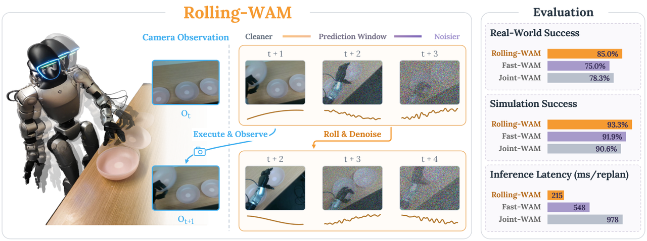
Figure 1: Rolling-WAM overview — a rolling window of staggered noise levels; retained chunks continue denoising as the window advances.
2. Method: Rolling Denoising
2.1 Window Structure
The prediction window is partitioned into $W$ temporally aligned chunks $X_{1:W}$, where $X_j = (v^{(j)}, a^{(j)})$. Each action chunk $a^{(j)} = a_{t+(j-1)K : t+jK-1}$ contains $K$ actions, and its video chunk $v^{(j)}$ covers the same physical interval at the video sampling rate. Total horizon $H = WK$; execution advances one chunk at a time.
Let $\tau \in [0,1]$ parameterize denoising progress within one replanning cycle, decreasing from $1$ to $0$. The base noise schedule $\sigma(\cdot)$ is monotonically increasing, with $\sigma(1)=1$ (pure Gaussian) and $\sigma(0)=0$ (clean data).
2.2 Two Modes
(a) Rolling mode. The first chunk must be clean at cycle end; every other chunk must land exactly on the starting noise level of the position it will occupy after the shift. Chunk $j$ gets:
$$\sigma^{\text{rolling}}_j(\tau) = \sigma\!\left(\frac{j-1+\tau}{W}\right),\qquad j=1,\dots,W$$
As $\tau$ goes from $1$ to $0$, chunk $j$ moves from $\sigma(j/W)$ to $\sigma((j-1)/W)$. The first chunk becomes clean while later chunks retain progressively more noise. The crucial hand-off condition:
$$\sigma^{\text{rolling}}_{j+1}(0) = \sigma^{\text{rolling}}_{j}(1),\qquad j=1,\dots,W-1$$
In words: once the first chunk is removed, every retained chunk is already at exactly the starting noise level of its new position — no extra processing needed. Appending a fresh chunk at $\sigma=1$ restores the configuration for the next cycle.
(b) Initialization mode. At episode start there is nothing to inherit, so the whole window starts from Gaussian noise:
$$\sigma^{\text{init}}_j(\tau) = \sigma\!\left(\min\left(1,\ \tau + \frac{j-1}{W}\right)\right)$$
All chunks start at $\sigma=1$; nearer chunks begin denoising earlier while distant ones stay at pure noise until their turn. At completion $\sigma^{\text{init}}_j(0) = \sigma^{\text{rolling}}_j(0)$: the first chunk is executable and the rest enter rolling mode after the shift.
2.3 Sampling and Execution: Why It Saves
Allocate $N$ total denoising steps per chunk, choosing $N$ as a multiple of $W$ for even distribution. Initialization uses $\Delta\tau = -1/N$ and needs $N$ steps to reach rolling mode; every subsequent steady-state cycle needs only $N/W$ steps to produce the next executable chunk (each step $\Delta\tau = -W/N$).
Each denoising step jointly updates the whole window. Given predicted flow velocity $f_{\theta,j}$, the Euler update is:
$$\tilde{X}_j \leftarrow \tilde{X}_j + \left[\sigma_j(\tau+\Delta\tau) - \sigma_j(\tau)\right] f_{\theta,j}\!\left(\tilde{X}_{1:W}, \sigma; c_t\right)$$
Once the first chunk is clean the robot executes its $K$ actions, the window slides — remove the executed chunk, retain the rest, append a Gaussian-noise chunk — and the robot acquires the latest camera observation to condition the next cycle.
V1/A1 → clean, executable"] --> E1["Execute A1
acquire new observation"] E1 --> B1["Cycle 2: shift window
retained chunks keep denoising
append Gaussian chunk"] B1 --> B2["Only N/W = 2 steps
→ next executable chunk"] B2 --> B3["... steady-state loop ..."]
One counterintuitive but important point: every chunk still traverses all $N$ denoising steps before execution — the computation is merely spread across replanning cycles. Moreover, with $N$ fixed and enough GPU parallelism for the extended window, a larger window actually lowers steady-state latency. The paper stresses that this route is orthogonal to Fast-WAM / Efficient-WAM-style optimizations and can be combined with them.
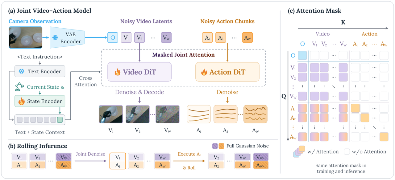
Figure 2: Framework — (a) masked joint attention across video/action experts, (b) rolling inference window shift, (c) the same attention mask in training and inference.
2.4 Architecture and Attention Mask
The model is an MoT: a pretrained video DiT (initialized from Wan2.2-TI2V-5B, reusing its text encoder and VAE) plus a lightweight action Transformer (30 layers, hidden dim $d_a = 1024$, ~1B parameters, backbone initialized by interpolating the video expert's weights). Both experts and the proprioceptive encoder are trained jointly; VAE and text encoder stay frozen.
The attention mask is the crux:
- Every action chunk can attend to visual features across the entire prediction window — this is what lets actions see a shared, evolving visual future extending beyond their own execution interval;
- Direct action-to-action attention is restricted to the same chunk;
- Video tokens do not attend to action tokens.
The same mask is used in both training and inference, avoiding train/deploy mismatch. Video and action tokens are modulated by their chunk-wise noise levels so predictions at different refinement stages can be processed jointly.
2.5 Training Objective
Trained with flow matching. For each window, sample $\tau \sim \mathcal{U}(0,1)$ and pick rolling or initialization mode with probabilities $\beta$ and $1-\beta$ (0.8 / 0.2). Noisy targets:
$$\tilde{X}_j = (1-\sigma_j)X_j + \sigma_j \epsilon_j,\qquad \epsilon_j \sim \mathcal{N}(0, I)$$
Video and actions use independent Gaussian samples; the network predicts conditional velocities with target $\epsilon_j - X_j$. For modality $q \in \{v,a\}$, the per-chunk loss is:
$$\ell^q_j = \left\| \left[f^q_\theta\!\left(\tilde{X}_{1:W}, \sigma; c_t\right)\right]_j - \left(\epsilon^q_j - X^q_j\right) \right\|_2^2$$
and the joint objective:
$$\mathcal{L} = \mathbb{E}\left[\frac{1}{W}\sum_{j=1}^{W} b_j\, w(\sigma_j)\left(\lambda_v \ell^v_j + \lambda_a \ell^a_j\right)\right]$$
where $w$ weights noise levels, $\lambda_v, \lambda_a$ balance modalities (both 1), and the activity mask $b_j$ excludes initialization chunks still held at pure noise. Training on both modes equips one model to both initialize the window and continue refining it during closed-loop execution.
2.6 Implementation Details: A Copyable Configuration
The paper is refreshingly specific. Video expert from Wan2.2-TI2V-5B with its pretrained text encoder and VAE reused; action expert with 30 layers, $d_a = 1024$, ~1B parameters, backbone not randomly initialized but interpolated from the video expert's weights — giving it visual priors from the start. Both experts plus the proprioceptive encoder are trained; VAE and text encoder frozen.
AdamW, learning rate $10^{-4}$, weight decay $10^{-2}$, 5% linear warmup then cosine decay, BF16 mixed precision. Video and action losses averaged separately with $\lambda_v = \lambda_a = 1$. Initialization and rolling modes sampled at 0.2 / 0.8. Both modalities share the shifted schedule $\sigma(\tau) = \rho\tau / [1+(\rho-1)\tau]$ with $\rho = 5$, train and inference alike. Defaults $N=10$, $W=5$, $K=16$, so steady state is just $N/W = 2$ steps per cycle; classifier-free guidance scale 1 (i.e., no CFG).
What this configuration means in one line: the model's total prediction horizon is $H = WK = 80$ actions, yet each update costs only 2 denoising steps. That arithmetic is where the 4.5× comes from — Joint-WAM runs a full denoising pass for 16 actions every cycle; Rolling-WAM runs 2 steps over an 80-action window.
2.7 Sitting It Among Contemporaries
Placed in the 2026 landscape of WAM acceleration, the map is clear:
| Route | Representative | Core idea | Cost |
|---|---|---|---|
| Remove test-time imagination | Fast-WAM | No future-video generation at deployment; keep it only as training supervision | Loses explicit visual prediction |
| Cache future context | Faster-WAM | Single video-expert pass extracts future context, cached for action denoising | Context stops updating with observations |
| Model / sampler compression | Efficient-WAM, Flash-WAM | Smaller model and visual tokens, fewer denoising steps, modality-aware consistency distillation | Capacity or quality limited |
| Context reuse | MotusBrain, AHA-WAM | Recycle visual features after partial joint denoising; share asynchronously refreshed visual context across action updates | Needs extra routing / refresh machinery |
| Execution overlap | RTC (real-time chunking) | Overlap inference with execution; action inpainting aligns successive chunks | Does not reduce total compute |
| Amortized denoising (this work) | Rolling-WAM | Spread joint denoising across replanning cycles with staggered in-window noise | Retained predictions may lag rapid scene changes |
Closest relatives are action-only rolling diffusion policies (Streaming Diffusion Policy, RNR-DP), which also maintain partially denoised action buffers but handle actions only and are evaluated on task-specific policies at smaller scale. Rolling-WAM's advance is extending the rolling mechanism to couple world modeling with action generation, letting action tokens attend to partially denoised visual futures, and evaluating across broader multitask settings.
Why Keeping Visual Imagination Matters
Worth stating separately. The Fast-WAM line effectively concludes that "test-time future imagination is unnecessary" — if true, that weakens the core distinction between WAMs and ordinary VLAs. Rolling-WAM offers a more constructive answer: it is not that future imagination is useless, it is that "regenerating the whole future from scratch every cycle" is too expensive. Once denoising is amortized, a model that keeps future-video generation not only beats Fast-WAM on speed (215 ms vs 548 ms) but also scores higher on RoboTwin and real-world tasks. That is a positive signal for the WAM line as a whole.
3. Experiments
3.1 Setup
Three settings: LIBERO (Spatial/Object/Goal/Long suites; one policy across all four; 10 epochs; 50 rollouts per task), RoboTwin 2.0 (50 bimanual tasks in Clean and Randomized settings; 2,500 clean + 25,000 randomized demonstrations; 100 rollouts per task per setting), and a real Unitree G1 (Doll Placement, Plate Stacking, Bead Pouring; 320×224 egocentric RGB plus a 43-D state; outputs 78-D actions = a 64-D SONIC motion latent plus 7-D commands per hand; 50 demonstrations per task at 10 Hz, 7,500 training steps, 20 trials per task).
Defaults: $N=10$ steps/chunk, $W=5$ chunks, $K=16$ actions/chunk, so steady state is $N/W = 2$ steps per cycle. Noise schedule $\sigma(\tau) = \rho\tau/[1+(\rho-1)\tau]$ with $\rho=5$; CFG scale 1. Only benchmark demonstrations are used — no additional embodied pretraining.
3.2 LIBERO: No Regression
| Method | Pretraining | Spatial | Object | Goal | Long | Average |
|---|---|---|---|---|---|---|
| $\pi_0$ | ✓ | 96.8 | 98.8 | 95.8 | 85.2 | 94.1 |
| $\pi_{0.5}$ | ✓ | 98.8 | 98.2 | 98.0 | 92.4 | 96.9 |
| Motus | ✓ | 96.8 | 99.8 | 96.6 | 97.6 | 97.7 |
| LingBot-VA | ✓ | 98.5 | 99.6 | 97.2 | 98.5 | 98.5 |
| Fast-WAM | ✗ | 98.2 | 100.0 | 97.0 | 95.2 | 97.6 |
| Joint-WAM | ✗ | 99.6 | 99.4 | 98.2 | 96.8 | 98.5 |
| Rolling-WAM (Ours) | ✗ | 98.2 | 98.0 | 98.2 | 97.8 | 98.1 |
98.1% — within 0.4 points of the joint leaders LingBot-VA and Joint-WAM (98.5%), above Motus (97.7%) and Fast-WAM (97.6%), with consistent 97.8–98.2% across the four suites.
3.3 RoboTwin 2.0: Actually Better
| Method | Pretraining | Clean | Randomized | Average |
|---|---|---|---|---|
| $\pi_0$ | ✓ | 65.9 | 58.4 | 62.2 |
| $\pi_{0.5}$ | ✓ | 82.7 | 76.8 | 79.8 |
| Motus | ✓ | 88.7 | 87.0 | 87.8 |
| LingBot-VA | ✓ | 92.9 | 91.5 | 92.2 |
| Fast-WAM | ✗ | 91.9 | 91.8 | 91.8 |
| Joint-WAM | ✗ | 90.8 | 90.3 | 90.6 |
| Rolling-WAM (Ours) | ✗ | 93.5 | 93.0 | 93.3 |
93.3% average — the highest among all compared methods — with only a 0.5-point gap between Clean and Randomized. Notably, Rolling-WAM uses no embodied pretraining at all yet beats the pretrained LingBot-VA (92.2%). The paper leans toward an explanation that co-refining current and future predictions may itself yield better action consistency.
3.4 Latency: The Headline
Measured on a single NVIDIA A100 under the RoboTwin 2.0 setting at 384×320: steady-state replanning latency including visual encoding and denoising with CUDA synchronization, excluding warm-up and initialization, with no torch.compile, TensorRT or custom CUDA kernels. All three methods execute 16 actions per cycle.
| Method | Steady-state replan latency (ms) | vs Rolling-WAM |
|---|---|---|
| GR00T N1.7 | 285 | 1.33× slower |
| $\pi_{0.5}$ | 296 | 1.38× slower |
| Fast-WAM | 548 | 2.5× slower |
| Joint-WAM | 978 | 4.5× slower |
| Rolling-WAM | 215 | — |
Two easily missed details:
- It keeps future-video generation yet is faster than both VLA baselines (215 ms vs 285/296 ms).
- It maintains an 80-action prediction window while baselines predict 16 — lower latency while refining a longer future at each update.
Window sweep ($W$ from 1 to 8; Rolling-WAM uses $H = 16W$, baselines fixed $H=16$; total budget $N = W\lfloor 16/W \rfloor$): at $W=5$, Rolling-WAM needs 322 ms vs 832 ms (Fast-WAM) and 1529 ms (Joint-WAM) — 2.58× and 4.75×. The curve flattens at $W=6$–$8$ where rolling steps stay at 2 per cycle.
3.5 Real-World Unitree G1
| Method | Doll Placement | Plate Stacking | Bead Pouring | Average |
|---|---|---|---|---|
| $\pi_{0.5}$ | 55.0 | 70.0 | 60.0 | 61.7 |
| GR00T N1.7 | 75.0 | 65.0 | 60.0 | 66.7 |
| Fast-WAM | 85.0 | 80.0 | 60.0 | 75.0 |
| Joint-WAM | 70.0 | 100.0 | 65.0 | 78.3 |
| Rolling-WAM (Ours) | 85.0 | 100.0 | 70.0 | 85.0 |
85.0% average — best of the five (Joint-WAM 78.3%, Fast-WAM 75.0%) — from a single policy trained across all three tasks. The paper also offers a telling qualitative note: execution across action-chunk boundaries is visibly more continuous with Rolling-WAM; pauses with Joint-WAM are more apparent and sometimes interrupt task progress. That sentence is arguably the strongest argument in the whole paper — latency is not just a number, it shows up as whether the robot stutters.
3.6 Ablations
| Variant | RoboTwin (6 tasks) | LIBERO |
|---|---|---|
| Full rolling (default, no cross-chunk action attn.) | 78.2 | 98.1 |
| With cross-chunk action attention (A2A) | 76.3 | 97.9 |
| Constant noise, replacement ratio $p=0.2$ | 74.7 | 97.9 |
| Constant noise, $p=0.5$ | 73.0 | 97.1 |
| Random noise, $p=0.2$ | 75.3 | 97.0 |
| Random noise, $p=0.5$ | 78.5 | 97.3 |
Three conclusions:
- Bigger windows are not better. On six RoboTwin tasks, $W=5$ peaks at 78.2%, $W=3$ gives 77.3%, $W=8$ drops to 69.5%. The conjecture: more distant visual predictions are less constrained by the current observation and may offer limited guidance for the imminent chunk — long windows can actively hurt.
- Training with the inference-matching staggered schedule is best. Random($p=0.5$) lifts RoboTwin to 78.5% but drops LIBERO to 97.3%; no alternative improves both, so the full rolling schedule is kept for all non-initialization samples.
- Action chunks should coordinate through the visual window, not directly. Adding A2A gives 76.3% / 97.9% versus 78.2% / 98.1% for within-chunk attention.
4. Our Take
The methodological value here exceeds the metric value. At heart it identifies the discarding inherent in receding-horizon control as wasted computation, borrows a ready-made answer from rolling diffusion, and fits it onto joint video-action models. The idea is clean, the implementation change is modest, the gain is a solid constant factor (4.5×), and it is orthogonal to Fast-WAM / Efficient-WAM / distillation-style speedups, so it stacks.
Points worth particular attention:
- Amortize rather than amputate. The dominant way to accelerate WAMs had been to remove test-time future generation — conceding that visual imagination is too expensive. Rolling-WAM shows that with a better ordering of denoising, imagination can stay, and still run 2.5× faster than Fast-WAM which drops it entirely.
- Beating the pretrained LingBot-VA on RoboTwin suggests cross-chunk visual context supplies real extra signal, not just saved FLOPs.
- "A2A makes it worse" is a nicely counterintuitive result: action chunks should not talk to each other directly but coordinate through a shared visual future — implying visual prediction acts precisely as the coordination medium.
- The real-world note (more continuous execution at chunk boundaries) argues latency's importance better than any table.
The Physics Behind Window Size
One easy-to-skip conversion: $H = WK = 5 \times 16 = 80$ actions means at 10 Hz the model is continuously imagining roughly 8 seconds ahead; at $W=8$ that becomes 12.8 seconds. A natural reading of the ablation drop past $W=5$ is: beyond some span, the imagined visual future has drifted from what will actually happen far enough to be harmful — attending to it is like reading an increasingly unreliable map.
This also explains why direct cross-chunk action attention hurts (78.2% → 76.3%). Retained far-future action predictions are lower quality still — they have not really been conditioned on observations yet. Routing coordination through the shared visual future substitutes a comparatively reliable medium for an unreliable direct link. The design choice is reasoned, not incidental.
An Engineering Caveat
That 215 ms comes from a single A100 with no torch.compile, TensorRT, or custom CUDA kernels — a deliberately conservative baseline. Real deployments with compilation, a smaller video expert, or more aggressive window settings have obvious headroom. Conversely, the 978 ms it is compared against is equally unoptimized, so 4.5× is a credible relative claim, but neither absolute number should be quoted as a deployment floor or ceiling.
Also, $W$ and $K$ are clearly task-dependent: $W=5$ optimal and $W=8$ down to 69.5% were measured at 10 Hz control with 16 actions per chunk. At higher control frequencies or with longer action chunks the optimum will likely differ — a limitation the authors acknowledge. Treat these as hyperparameters to re-sweep rather than defaults.
Reading It Against ME-U0
Read alongside Li Auto's contemporaneous ME-U0 (arXiv:2609.25627), the division of labor is neat: ME-U0 asks how understanding, prediction and control unify architecturally (subtask + affordance conditioning of joint visual-action generation), while Rolling-WAM asks how that joint denoising can be afforded in a closed loop. One adds capability, the other cuts cost — orthogonal directions, and Rolling-WAM explicitly notes it composes with model- and system-level optimizations such as ME-U0's. Together the two papers sketch the main battlefields of the 2026 WAM line.
Limitations are stated plainly: window and chunk sizes warrant further exploration across tasks with different dynamics and control frequencies; despite observation feedback, retained predictions may lag rapid scene changes and misguide action generation, especially with long windows; adaptive window management and asynchronous execution are named next steps.
5. Resources
- Paper: arXiv:2609.30247
- Project page: https://rolling-wam.github.io/
- Affiliations: USC (Physical Superintelligence Lab), Brown University, Fudan University, Toyota Research Institute
- Support: NSF CPS #2434460