PAPER DEEP DIVE
Depth Anything V4: Dynamic 4D Scene Reconstruction via Riemannian Flow Matching on 4D Gaussian Splatting
WITHDRAWN / archival entry: arXiv marks this paper as withdrawn by its authors (v2, 20 Aug 2026, 1 KB record, comment: “Major errors in research”); it is kept here for critical reading only. The paper itself proposes Depth Anything V4 (DAV4), dynamic 4D scene reconstruction from monocular video by defining Riemannian Flow Matching (RFM) directly on the non-Euclidean manifolds of 4D Gaussian Splatting parameters (scale, rotation, opacity), so every intermediate state on the probability path remains valid without post-hoc projection. A deterministic MLP baseline sharing the same data, architecture and test-time optimization (TTO) protocol isolates the contribution: MLP+TTO scores 0.762 F-score versus 0.806 for RFM+TTO, a +0.044 isolated gain, while Euclidean flow matching with projection reaches only 0.684 with 12.3% invalid Gaussians. Pre-training costs 360 GPU-hours and amortizes only beyond roughly 10,000 scenes; uncertainty is quantified via negative Gaussian log-likelihood and expected calibration error; no human-annotated depth labels are used as training losses.
Depth Anything V4: Riemannian Flow Matching on the Parameter Manifolds of 4D Gaussian Splatting
Withdrawal notice (read first)
This paper (arXiv:2608.18388) has been withdrawn by its authors. The arXiv abstract page carries the notice "This paper has been withdrawn by Jiaming Fan"; version 2 (20 Aug 2026) is a 1 KB withdrawal record whose stated comment is "Major errors in research", and that version carries no license. This entry is kept as an archival, critical-read record only. Every method description, equation and experimental number below is transcribed faithfully from the surviving v1 full text and does not imply that this site endorses the claims as still valid; any citation should state the withdrawal. The declared project repository returns 404 and the author account hosts no public repositories, so none of the reported numbers can currently be independently reproduced.
Paper: Depth Anything V4: Dynamic 4D Scene Reconstruction via Riemannian Flow Matching on 4D Gaussian Splatting | Authors: Jiaming Fan, Jian Lu, Jinling Jia, Chenbin Zhang | Affiliation: College of Artificial Intelligence and College of Automation, Nanjing University of Posts and Telecommunications | Link: https://arxiv.org/abs/2608.18388 | Code: not available (the declared project page https://github.com/fjm123456789/Depth-Anything-4 returns 404) | Status: withdrawn (v2, 20 Aug 2026)
One-sentence summary
DAV4 places the probability path of flow matching directly on the non-Euclidean manifolds of 4D Gaussian Splatting parameters (scale, rotation, opacity) so that every intermediate sample stays valid, and isolates a +0.044 F-score gain of the formulation against a deterministic regression baseline with identical data, architecture and test-time optimization; the authors nevertheless withdrew the paper two days after submission, citing major errors in the research.
Background and motivation
The Depth Anything family (V1, V2, V3) established feed-forward monocular depth estimation as a discriminative regression problem: semi-supervised learning, synthetic-data refinement, then multi-view geometric reasoning, all producing per-pixel point estimates at roughly 38 ms per frame. The trade-off is deliberate. There is no temporal model, no predictive distribution, and no volumetric scene representation. That is acceptable for real-time perception, but offline content creation, 3D archiving and dynamic scene understanding need more than a depth map.
The alternative route is per-scene optimization. 4D Gaussian Splatting, Deformable-GS and Dynamic 3DGS each optimize a time-deforming set of Gaussians for one scene at a time, requiring thousands of iterations (this paper reports about 2100 ms per scene for fully optimized 4D-GS) and restarting from scratch for every new scene. The cost never amortizes across scenes, which rules out large video corpora.
Generative priors offer a third option: learn the mapping from observations to scene representations into network weights, so inference is sampling. Flow matching is a simulation-free training paradigm for continuous normalizing flows, and its Riemannian generalization (RFM) allows probability paths on curved manifolds. The obstacle is that 4DGS parameters do not live in Euclidean space.
Scales must stay positive, rotations must stay on SO(3), and opacities must stay inside the open interval (0,1). Linear interpolation between two Gaussian sets in Euclidean space leaves these constraints, producing negative scales or non-unit quaternions that must be rescued by post-hoc projection (clipping, Gram-Schmidt). Projection breaks the continuity of the probability path and decouples the training target from the sampling trajectory. Figure 1 states the intuition visually: the Euclidean chord exits the manifold, the geodesic never does.
The paper therefore defines the conditional vector field of RFM on the product manifold of 4DGS parameters, making training target, sampling path and parameter constraints mutually consistent. Unlike V1 to V3, DAV4 positions itself as an offline high-fidelity reconstructor (420 ms per scene) rather than a real-time estimator. Its most notable experimental stance is the acknowledgment that pre-training plus test-time optimization alone already yields large gains, so a deterministic MLP baseline is built to separate the formulation's contribution from the engineering contribution.
Preliminaries: parameter manifolds and Riemannian flow matching
A 3DGS field consists of N Gaussians, each carrying a center $\bm{\mu}\in\mathbb{R}^{3}$, a scale $\mathbf{s}\in\mathbb{R}_{>0}^{3}$, a rotation $\mathbf{q}\in\mathrm{SO}(3)$, spherical-harmonic colors $\mathbf{c}$ and an opacity $\alpha\in(0,1)$. The 4D extension follows 4D-GS and decomposes the scene at video time $\tau$ into a static base field plus a time-conditioned residual,
$$\mathcal{S}(\mathbf{x},\tau)=\mathcal{S}_{3D}(\mathbf{x})\oplus\Delta_{\bm{\phi}}(\mathbf{x},\tau),\quad \Delta_{\bm{\phi}}(\bm{\mu}_{i},\tau)=\mathrm{MLP}_{\bm{\phi}}(\gamma(\bm{\mu}_{i}),\gamma(\tau)),$$
where $\gamma(\cdot)$ denotes positional and temporal frequency encodings and the residual is bounded by $\tanh$. The decomposition compresses dynamics into a bounded residual field while the base field carries static structure and identity across frames.
Flow matching on a manifold $\mathcal{M}$ defines the conditional probability path by geodesic interpolation between a noise sample $\mathcal{G}_z$ and a target sample $\mathcal{G}_1$, together with the closed-form conditional vector field
$$\mathcal{G}_{t}=\mathrm{Exp}_{\mathcal{G}_{z}}\!\left(t\cdot\mathrm{Log}_{\mathcal{G}_{z}}(\mathcal{G}_{1})\right),\quad u_{t}(\mathcal{G}_{t}\mid\mathcal{G}_{1},\mathcal{G}_{z})=\frac{\mathrm{Log}_{\mathcal{G}_{t}}(\mathcal{G}_{1})}{1-t},$$
and trains the network field $v_{\bm{\theta}}$ to regress it: $\mathcal{L}_{\text{RFM}}=\mathbb{E}\left[\lVert v_{\bm{\theta}}(\mathcal{G}_{t},t)-u_{t}\rVert^{2}_{\mathcal{M}}\right]$. Because $u_t$ is closed-form, training never solves an ODE, which is the main engineering advantage over diffusion-style training.
Each non-Euclidean component gets its own manifold operation. Scales are interpolated as a geometric mean in log coordinates, $\tilde{\mathbf{s}}=\log\mathbf{s}$ with $\mathbf{s}_{t}=\mathbf{s}_{z}^{1-t}\mathbf{s}_{1}^{t}$, keeping every intermediate scale positive; rotations follow SO(3) geodesics through exponential and logarithmic maps; opacities are mapped to the whole real line by the logit $\tilde{\alpha}=\log(\alpha/(1-\alpha))$ and interpolated linearly there. Appendix B sketches the correctness argument: the conditional field $u_t$ is the gradient of the Gaussian negative log-likelihood on the tangent space, so matching it minimizes the KL divergence between model and target distributions.
Method
Representation. The output object is a 4DGS field evolving over video time, using the static-base-plus-residual decomposition above with a bounded residual MLP over frequency-encoded position and time. Choosing a decomposition instead of per-frame independent reconstruction builds temporal consistency into the representation: the same base Gaussians keep their identity in every frame, and motion lives only in the bounded increments.
Riemannian flow matching prior. The prior network is trained with the conditioned version of the RFM objective,
$$\mathcal{L}_{\text{RFM}}=\mathbb{E}\left[\left\lVert v_{\bm{\theta}}(\mathcal{G}_{t},t,f_{\text{img}},\gamma(\tau))-u_{t}\right\rVert^{2}_{\mathcal{M}}\right],$$
so the vector field is conditioned on flow time $t$, frozen DINOv2-L image features $f_{\text{img}}$ and video time $\tau$. The norm is taken on the product manifold as a sum of tangent-space norms: Euclidean in log-scale and logit-opacity coordinates, SO(3) tangent norm for rotations. Conditioning is what separates this prior from unconditional Gaussian generation: it models "what the scene should look like given this video".
Deterministic MLP baseline (the anchor of the controlled study). To isolate RFM, the flow matching objective is replaced by plain L2 regression to the teacher targets,
$$\mathcal{L}_{\text{MLP}}=\mathbb{E}_{\mathcal{G}_{1}\sim p_{\text{teacher}}}\left[\left\lVert \mathrm{MLP}_{\bm{\phi}}(f_{\text{img}},\gamma(\tau))-\mathcal{G}_{1}\right\rVert^{2}\right],$$
while backbone, Perceiver, decoder heads, pre-training data, augmentations, schedules and the TTO protocol stay identical (Appendix C). The only variable is the loss. This baseline gives the later +0.044 an explicit attribution target: not more parameters, not more data, but the probabilistic formulation itself, at least as v1 claims.
Self-supervised teacher. Flow matching needs target samples $\mathcal{G}_1$, and annotated 4DGS does not exist. The teacher is a 4DGS head trained with purely self-supervised losses,
$$\mathcal{L}_{\text{teacher}}=\lambda_{r}w(t)\mathcal{L}_{\rm render}+\lambda_{e}\mathcal{L}_{\rm equiv}+\lambda_{f}\mathcal{L}_{\rm flow}+\lambda_{\rm scale}\mathcal{L}_{\rm scale}+\lambda_{\rm reg}\mathcal{L}_{\rm reg}.$$
The five terms divide the labor: a rendering loss for photometric consistency; an SE(3)-equivariance loss with rigidity scores for geometric priors; a RAFT optical-flow consistency loss to disambiguate temporal dynamics; a scale regularization that borrows median depth from Depth Anything V2 to fix metric scale (disclosed by the authors as weak supervision); and a Gaussian regularizer against degenerate primitives. The paper repeatedly stresses that no human-annotated depth enters the training losses.
Test-time optimization. Sampled fields are refined by adding the rendering-loss gradient to the right-hand side of the ODE as a guidance term,
$$\frac{d\mathcal{G}_{t}}{dt}=v_{\bm{\theta}}(\mathcal{G}_{t},t,f_{\text{img}},\gamma(\tau))+w_{\text{guide}}\cdot\nabla_{\mathcal{G}}\mathcal{L}_{\text{render}}(\mathcal{G}_{t}).$$
Every TTO-based method (4D-GS+TTO, MLP+TTO, RFM+TTO) shares one protocol: 20 gradient steps, learning rate $10^{-3}$, Adam, identical rendering loss. Protocol uniformity is the precondition for the controlled study and the most commendable part of the experimental design.
Architecture. Each Gaussian is encoded into a 64-dimensional latent $\mathbf{z}_{i}=\mathrm{Enc}_{\rm gauss}(\cdot)$; a Perceiver (4 layers, hidden 256) compresses the variable-size set into M=512 fixed tokens $\mathbf{H}$; cross-attention reads the global tokens back per Gaussian, $\mathbf{h}_{i}=\mathrm{CrossAttn}(\mathbf{z}_{i},\mathbf{H}_{\rm out})$; and a multi-head MLP emits increments $\Delta\mathcal{G}_{i}$ for position, scale, quaternion and opacity (Figure 2). The frozen DINOv2-L backbone supplies semantic features, and the vector-field estimator is a 4-layer Transformer whose conditions enter through sinusoidal embeddings.
flowchart TB
    V[Monocular video frames] --> DINO[Frozen DINOv2-L backbone]
    DINO --> PER[Perceiver: variable set to M=512 tokens]
    PER --> VF[Transformer vector field estimator]
    EMB[Sinusoidal embedding of flow time t and video time tau] --> VF
    VF --> COARSE[Coarse ODE stage: 10 steps, global layout]
    COARSE --> FINE[Fine ODE stage: 20 steps, local detail]
    FINE --> GS[4DGS field: position, scale, quaternion, opacity]
    GS --> RENDER[Differentiable rendering loss]
    RENDER -. guidance gradient, weight 0.01 .-> FINE
    subgraph MFD[Probability path on parameter manifolds]
        SC[Scale: log-space geodesic]
        RO[Rotation: SO(3) Exp/Log geodesic]
        OP[Opacity: logit-space geodesic]
    end
    VF --> MFD
    MFD --> GS
Coarse-to-fine sampling. Algorithm 1 splits ODE integration into two stages: a coarse stage of 10 steps with step size $1/N_c$ that captures global layout, and a fine stage of 20 steps with halved step size that refines detail and optionally adds the task-loss guidance gradient at half weight ($w/2$, compensating the half step). The noise init $\mathcal{G}_0\sim\mathcal{N}(0,\mathbf{I})$ lives in tangent-space coordinates of each manifold, and the scene size is fixed at 100,000 Gaussians.
Uncertainty quantification. A generative prior yields distributions for free: K=10 independent ODE trajectories from different noise inits give a per-parameter empirical variance across samples. Calibration is reported as negative Gaussian log-likelihood (NGLL), computed directly in parameter space,
$$\mathrm{NGLL}=-\frac{1}{N}\sum_{i}\left[-\frac{1}{2}\log(2\pi\sigma_{i}^{2})-\frac{(\theta_{i}-\hat{\theta}_{i})^{2}}{2\sigma_{i}^{2}}\right],$$
with $\sigma_i^2$ the empirical variance, avoiding high-dimensional density estimation; ECE uses 10 equally spaced confidence bins with per-pixel confidence equal to the inverse variance.
Cost model. Pre-training costs 360 GPU-hours, i.e. $1.296\times10^{6}$ GPU-seconds, and per-scene inference takes 420 ms. Amortized cost per scene is $420+1.296\times10^{6}/N$ milliseconds: 1716 ms at N=1000, worse than per-scene optimization, but about 550 ms at N=10,000, which beats the 2100 ms of fully optimized 4D-GS. The authors accordingly draw the applicability boundary at offline batch processing above ten thousand scenes.
Experiments and interpretation
Evaluation covers four benchmarks: Dynamic-Sim (100 synthetic dynamic scenes with 4DGS ground truth), KITTI Dynamic (50 KITTI Tracking sequences with moving vehicles and pedestrians), and ETH3D plus ScanNet for novel-view synthesis. Pre-training uses unlabeled WebVid-10M video and unlabeled MegaDepth images. Table 1 is the experimental core: it decomposes the total gain into three attributable factors.
| Method | Pre-training | TTO | Dynamic-Sim F1 | KITTI F1 |
|---|---|---|---|---|
| 4D-GS (5000 iter) | No | No | 0.781 | 0.623 |
| 4D-GS (100 iter) | No | No | 0.702 | 0.552 |
| 4D-GS + TTO | No | Yes | 0.748 | 0.598 |
| MLP | Yes | No | 0.718 | 0.578 |
| MLP + TTO | Yes | Yes | 0.762 | 0.615 |
| RFM (DAV4) | Yes | No | 0.758 | 0.612 |
| RFM + TTO (DAV4) | Yes | Yes | 0.806 | 0.652 |
| Delta: TTO | +0.046 | +0.046 | ||
| Delta: pre-training | +0.014 | +0.017 | ||
| Delta: RFM | +0.044 | +0.037 |
Three readings matter. First, TTO alone is a strong baseline: 20 test-time steps lift under-optimized 4D-GS from 0.702 to 0.748 (+0.046), so any new method must clear that bar before claiming anything. Second, pre-training contributes only +0.014, showing that pouring data into a network does not automatically pay on this task. Third, the isolated RFM gain of +0.044 (+0.037 on KITTI) is more than three times the pre-training gain while both models share data, architecture and TTO protocol. An unfavorable reading must also be recorded honestly: RFM without TTO (0.758) is slightly below MLP with TTO (0.762), so the probabilistic prior and test-time optimization are complementary rather than substitutable.
On novel-view synthesis (Table 2), DAV4 beats randomly initialized 3D-GS under the same TTO budget by 2.79 dB on ETH3D (25.13 versus 22.34) and even surpasses fully optimized 3D-GS at 5000 iterations (24.12 dB); on ScanNet it leads the 20-step baseline by 2.24 dB (23.82 versus 21.58). LPIPS drops from 0.23 to 0.16, indicating that the gain is perceptual and not merely pixel alignment. The authors flag the inherent bias of this comparison themselves: 3D-GS starts from random initialization while DAV4 starts from a learned prior, an advantage that cannot be subtracted from the comparison.
| Method | ETH3D PSNR | ETH3D SSIM | ETH3D LPIPS | ScanNet PSNR | ScanNet SSIM | ScanNet LPIPS |
|---|---|---|---|---|---|---|
| 3D-GS (20 iter TTO) | 22.34 | 0.83 | 0.23 | 21.58 | 0.81 | 0.26 |
| 3D-GS (5000 iter) | 24.12 | 0.86 | 0.19 | 23.05 | 0.84 | 0.22 |
| MLP + TTO | 24.01 | 0.85 | 0.20 | 22.85 | 0.83 | 0.23 |
| DAV4 (RFM + TTO) | 25.13 | 0.88 | 0.16 | 23.82 | 0.86 | 0.19 |
The time-conditioning ablation (Table 3) supplies another clean causal reading: removing the video-time condition $\tau$ drops temporal consistency on KITTI Dynamic from 0.92 to 0.78 and F-score from 0.806 to 0.742. Without $\tau$ the model can only learn a time-averaged static prior, and motion cues never reach the vector field; the +0.14 consistency gain is the most direct evidence for the word "dynamic" in this paper. Figure 4 adds the efficiency view: DAV4 reaches its plateau of about 0.80 within the 20-step TTO budget, while per-scene 4D-GS needs more than 500 iterations to approach the same level.
The value of the geometric formulation is starkest in Table 5. Replacing RFM with Euclidean linear interpolation plus post-hoc projection (clipping scales positive, Gram-Schmidt for rotations) drops F-score to 0.684 with 12.3% of sampled Gaussians invalid before projection; the Riemannian version scores 0.806 with 0.01% invalid. In other words, roughly one eighth of the Euclidean path's samples need rescuing, and the rescue itself costs 0.122 of quality. The KITTI qualitative comparison (Figure 3) and the uncertainty heatmap (Figure 5, high variance on the moving car and occlusion boundaries, low variance on static background) support the qualitative claims of sharper boundaries and well-calibrated uncertainty.
| Method | F1 | Invalid Gaussians |
|---|---|---|
| Euclidean FM + projection | 0.684 | 12.3% |
| Riemannian FM (ours) | 0.806 | 0.01% |
For uncertainty (Table 4), multi-hypothesis sampling gives DAV4 an NGLL of -1.58 and an ECE of 0.058, clearly better than MC-Dropout (-0.82 / 0.18) and deep ensembles (-1.15 / 0.12). For downstream systems this means the model knows where it is unsure: high variance at occlusions and motion boundaries can drive rejection sampling or active view acquisition. The efficiency table (Table 6) draws the applicability boundary: 420 ms per scene is 11x slower than Depth Anything V3, and only beyond ten thousand deployed scenes does the amortized 550 ms make the pre-training investment pay off.
| Method | NGLL (lower better) | ECE (lower better) |
|---|---|---|
| MC-Dropout | -0.82 | 0.18 |
| Deep ensemble | -1.15 | 0.12 |
| DAV4 | -1.58 | 0.058 |
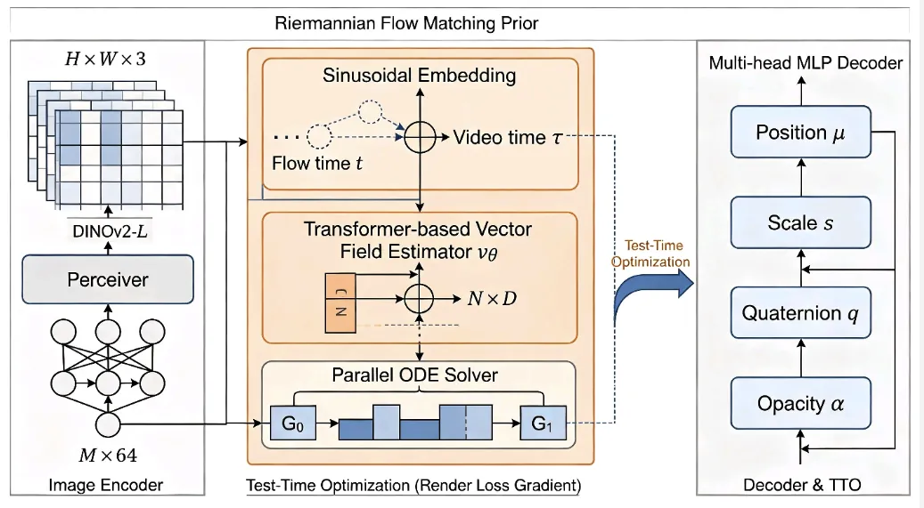
Figure 2: overall architecture. A frozen DINOv2-L backbone and a Perceiver produce latent tokens; the Riemannian flow matching prior estimates the vector field conditioned on flow time t and video time tau; the ODE solver generates Gaussians coarse-to-fine; test-time optimization refines them with a rendering loss.
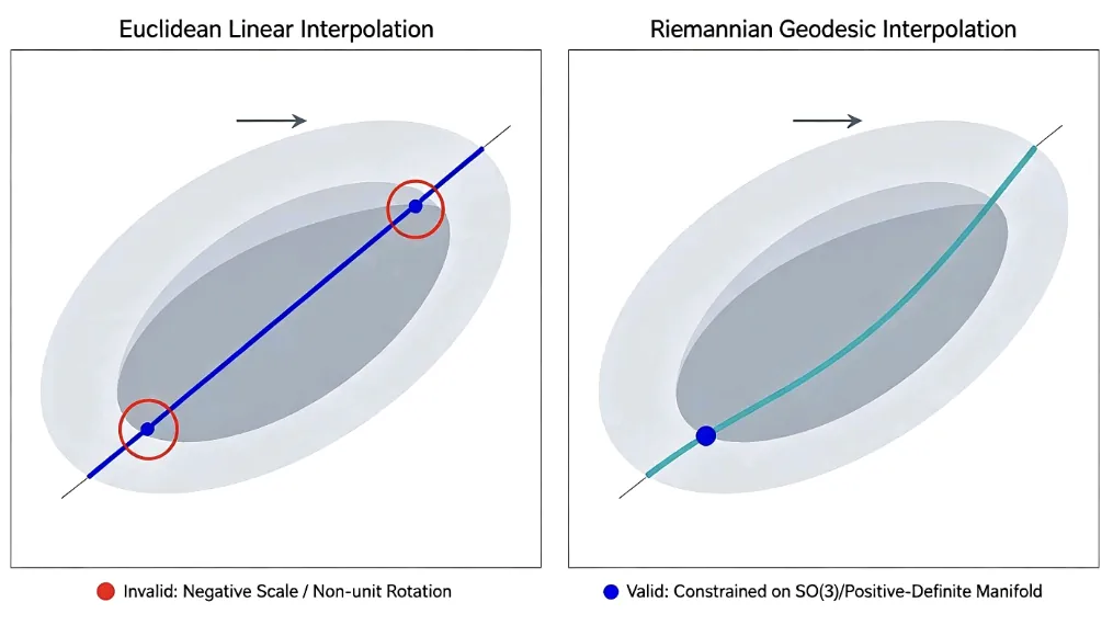
Figure 1: Euclidean linear interpolation (left) leaves the manifold and produces negative scales or non-unit rotations that need post-hoc projection; Riemannian geodesic interpolation (right) keeps every intermediate state valid.
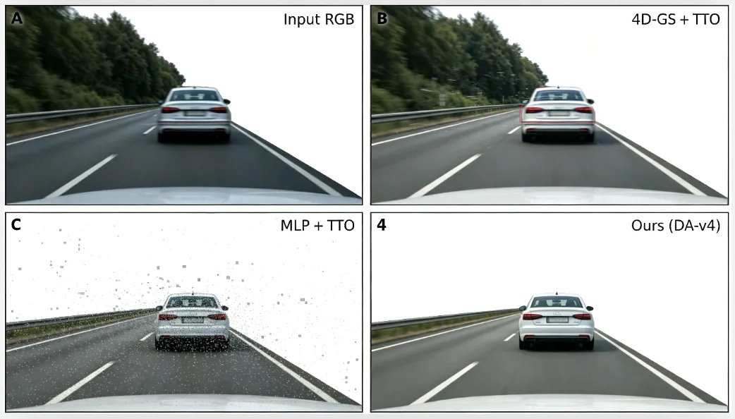
Figure 3: qualitative comparison on KITTI Dynamic. DAV4 (bottom right) shows sharper boundaries and fewer floaters than 4D-GS+TTO (top right) and MLP+TTO (bottom left).
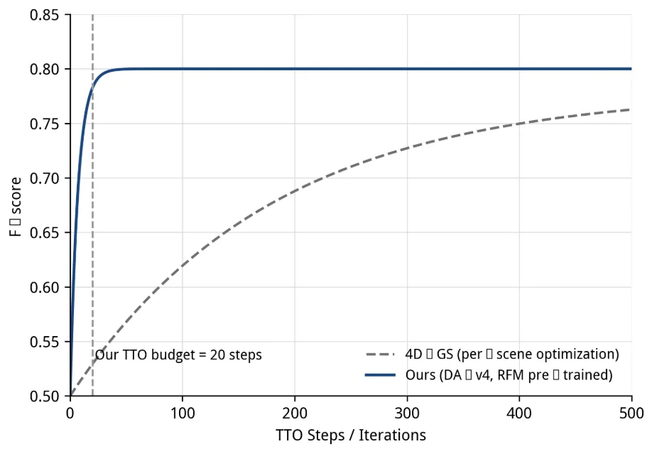
Figure 4: TTO convergence. DAV4 plateaus within the 20-step budget while per-scene 4D-GS needs more than 500 iterations.
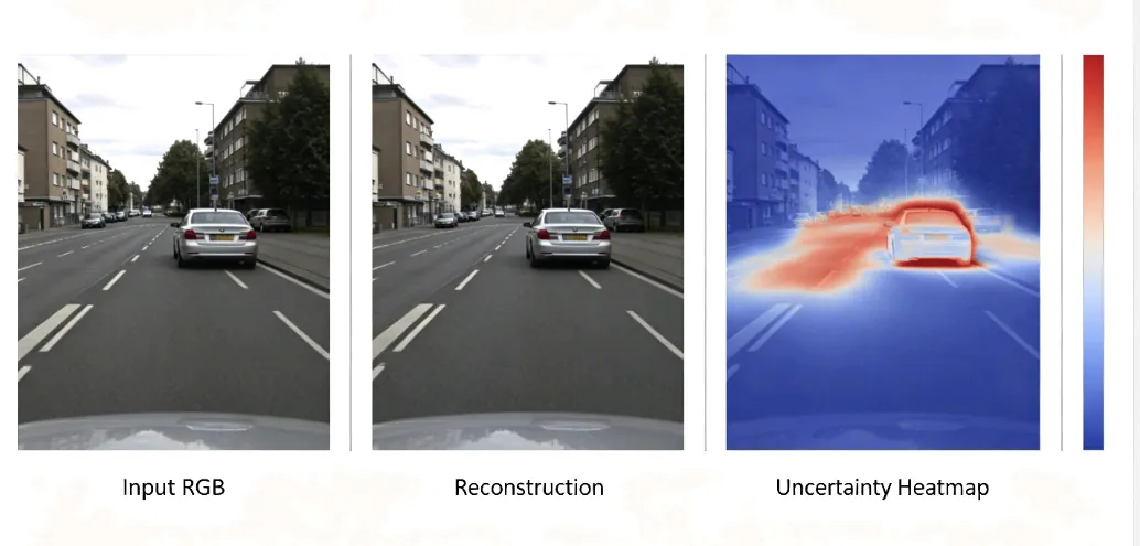
Figure 5: uncertainty visualization. Variance is high (red) on the moving vehicle and occlusions, low (blue) on static background.
Limitations
The authors state four limitations: 420 ms inference is unsuitable for real-time robotics and autonomous driving; pre-training demands 360 GPU-hours; the novel-view comparison against 3D-GS carries an inherent initialization bias (random versus pre-trained); and the rendering gradient is not a conservative vector field, so TTO guidance lacks a rigorous energy-based interpretation. The last admission is unusually honest: it concedes that the guidance term in Eq. (7) is a heuristic in mathematical terms.
Several further judgments must be recorded. First and heaviest: the authors withdrew the paper citing "major errors in research" without stating where the errors lie. With no code, no data, a self-built synthetic benchmark (Dynamic-Sim) and missing protocol details for KITTI Dynamic, every number in Tables 1 to 6 is currently an unreproducible claim; the +0.044 isolated gain should be read as an unverified proposition, not an established result. Second, the "identical architecture" promise of the controlled study rests on a single paragraph in Appendix C, with no table verifying parameter counts and initialization of the MLP baseline against RFM head by head. Third, approximating the predictive distribution by parameter variance across K=10 trajectories is a thin sample for a 10-bin ECE estimate, making tail-calibration claims fragile. Fourth, the scale regularization borrows median depth from Depth Anything V2; although disclosed as weak supervision, this sits in tension with the "no annotated depth" framing, since another depth model's output is doing real work in the loss.
Conclusion and outlook
Setting the withdrawal aside, the text poses a clean technical proposition: when a scene representation's parameters carry geometric constraints, a generative prior should respect those constraints on its probability path instead of walking in Euclidean space and projecting afterwards. The controlled-study design, quantifying TTO, pre-training and formulation gains separately as +0.046, +0.014 and +0.044, is a reporting standard that other prior-plus-optimization hybrids should copy, because it lets readers decide which part of the gain is worth paying for.
The withdrawal carries its own lesson: a paper that looks unusually careful in experimental design can still be retracted wholesale by its authors for unnamed major errors, and without reproducible artifacts the community cannot even locate the error. For future work, the manifold recipes themselves (log-space scales, SO(3) geodesics, logit opacities) remain valid engineering, with open references such as facebookresearch's riemannian-fm and flowmm available for verification; what needs re-establishment is the specific claim about how much those recipes buy on 4DGS parameters.
Golden quote
SOURCE LINKS