3D Point World Models: Point Completion Enables More Accurate Dynamics Learning

Authors: Skand Peri, Hung Nguyen, Chanho Kim, Li Fuxin, and Stefan Lee. Affiliation: Oregon State University. Paper: arXiv:2607.00148, first posted on June 30, 2026. This analysis uses version 2, dated October 7, 2026.

Project and code: The authors provide a project page and a GitHub repository. At the time of review, the repository snapshot contained only a README and an MIT license, with the README stating that code is “Coming soon.” The paper therefore supports a detailed review of the method and experiments, but not an independent source-level reproduction of the network, losses, planner, or data pipeline.

In one sentence: Completing segmented object point clouds before learning action-conditioned point velocities substantially improves long-horizon rollout accuracy, planning, novel task composition, and sim-to-real manipulation.

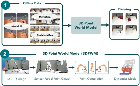
Figure 1: From one RGB-D view and robot joint angles, the system completes object geometry, forms a scene point cloud, and performs action-conditioned rollouts for planning.

Background and Motivation

A robot operating in a physical environment must do more than recognize the current scene. It must predict how a candidate action will alter that scene. World-model-based control turns this requirement into a learned transition function: receive an observation and an action, predict the next observation, and allow a planner to evaluate several possible futures. For manipulation, useful predictions include object centers, contact geometry, occluded volume, and the position of the end effector. A visually plausible future is insufficient if those quantities are wrong.

Most established world models learn dynamics in image or video space. They can represent rich appearance, but have two weaknesses in physical control. First, generated frames may obey visual statistics while violating rigid-body or contact constraints. Second, a real robot needs an action, not merely a future image. Inferring action from visual motion is ambiguous: the same apparent movement can require different torques or end-effector displacements when mass, friction, or grasp state differs. Pixel prediction therefore entangles scene evolution with a difficult inverse-control problem.

2.5D models add depth and surface normals, but still process these quantities as image-shaped features. Their geometry is only implicit, and predictions from different viewpoints may disagree. More importantly, a single camera sees only one side of an object. A dynamics network trained on partial geometry must simultaneously infer the missing shape and learn the physical transition. During recursive rollouts, an early completion error becomes part of the next input, so the mistake can grow into an incorrect object center, contact location, or collision estimate.

Another line of work builds world models directly on point clouds, particles, or Gaussian splats. This representation is closer to physical 3D state, but partial-view inputs remain a problem. The less visible side of an object is poorly constrained, particularly when another object or the gripper occludes it. Simulation can provide complete meshes during training, yet a deployed camera cannot. The resulting distribution shift makes a model that looked accurate in simulation less reliable on a real tabletop.

The paper addresses that mismatch with an explicit completion stage. It segments task-relevant objects, back-projects their depth into partial point clouds, completes each object, and combines the result with robot points generated from forward kinematics. The dynamics model then always sees complete object geometry. During simulation training, the same kind of complete point cloud comes directly from object meshes. Completion thus acts as a bridge between an easy training regime and a difficult real-world observation regime.

Problem Setup

At time $t$, the robot receives proprioception and a calibrated single-view depth observation. Let the joint configuration be $\mathbf{q}_t$. The system first converts the partial observation into a complete observation $\mathcal{O}^{\text{complete}}$, then learns a transition function $\mathcal{T}:\mathcal{O}^{\text{complete}}\times\mathcal{A}\rightarrow\mathcal{O}^{\text{complete}}$. The action $a_t$ is expressed in the end-effector frame. A sampling-based planner uses the learned transition function to score candidate action sequences.

Point identity must remain consistent across time. For point $j$, the model uses its position $\mathbf{x}_{t,j}$, current velocity $\mathbf{v}_{t,j}$, and previous velocity $\mathbf{v}_{t-1,j}$. In simulation, a canonical object point cloud can be transformed by rigid-body poses at every timestep, yielding exact point correspondences. In the real world, point tracking is needed to estimate similar correspondences. This supervision differs from comparing unordered point sets with Chamfer distance: the model is taught how each point moves, not only whether two shapes have nearby surfaces.

Planning uses model-predictive control with MPPI. The planner samples action sequences, rolls out predicted point clouds, computes a task cost on those predictions, and reweights the candidate trajectories. Because the state is already a 3D point cloud, a cost can directly use distances between the tool center point and an object, between an object center and a goal, or between manipulated geometry and obstacles. This interface resembles a simulator reward rather than an image reconstruction score.

Method

1. Constructing a complete scene from one view

The pipeline first asks a vision-language model to identify task-relevant objects and return two-dimensional point prompts inside their visible regions. SAM3 uses those prompts for open-vocabulary segmentation. Each mask is combined with the calibrated depth image and back-projected into a partial object point cloud. Segmenting objects separately lets the completion network focus on an individual shape and makes the resulting geometry easier to merge with robot points.

The completion component starts from ShapeNet-pretrained weights and is fine-tuned on YCB objects. The authors emphasize that their completion model does not require the center of the complete object. That property matters in a real scene because the center of unseen volume is not directly observable. The original completion pipeline assumes upright objects aligned along the vertical axis. Manipulated objects can have arbitrary orientation, so the paper augments both pretraining and fine-tuning with rotations around all three axes.

The point-cloud input is further degraded with random jitter to mimic depth-sensor noise. Boundary noise is cleaned using a procedure from prior work, and a median filter suppresses noisy depth values inside each object. These preprocessing choices are not cosmetic. Depth errors near glossy surfaces and occlusion boundaries can create points outside an object; completion can then infer an incorrect volume, which changes both the object center and the planned contact.

Robot geometry does not come from the camera. Given joint angles and the robot URDF, forward kinematics produces the robot point cloud:

$$\mathbf{P}_{t}^{\text{robot}}=\mathrm{FK}(\mathbf{q}_{t},\mathrm{URDF})$$

Since the action space is defined at the end effector, the implementation samples points only from the end-effector mesh. The complete scene is the union of these robot points and every completed task-relevant object:

$$\mathbf{P}_{t}=\mathbf{P}_{t}^{\text{robot}}\cup\bigcup_{\text{obj}}\mathbf{P}_{t}^{\text{obj}}$$

This union is essential. Object points alone do not reveal where the action originates, while end-effector points alone do not reveal the volume hidden behind the visible object surface. The combined cloud places both the cause and the affected geometry in one coordinate system.

Figure 2: The point-completion stage merges forward-kinematics and completed object clouds. The dynamics stage then predicts a velocity for every point.

flowchart LR
    A[Single RGB-D view and joint angles] --> B[VLM produces object point prompts]
    B --> C[SAM3 segments task-relevant objects]
    C --> D[Back-project depth to partial clouds]
    D --> E[Complete objects with ShapeNet pretraining and YCB fine-tuning]
    A --> F[Sample end-effector mesh through URDF and forward kinematics]
    E --> G[Merge complete scene cloud]
    F --> G
    G --> H[PTV3 encodes geometry and velocities]
    H --> I[Inject action and register token by cross-attention]
    I --> J[Propagate action effects with self-attention]
    J --> K[Decode per-point velocities and roll out recursively]
    K --> L[MPPI scores candidates on predicted point clouds]
    L --> M[Execute action chunk and capture the next view]
    M --> A
    

Diagram note: this is the paper-specific path from completion to dynamics and planning. The planner scores geometry produced by the world model rather than the visible partial cloud.

2. Point features and the PTV3 backbone

Every point is represented with position, current velocity, and previous velocity:

$$\mathbf{F}_{t}=[\mathbf{x}_{t},\mathbf{y}_{t},\mathbf{z}_{t},\mathbf{v}_{t},\mathbf{v}_{t-1}]$$

The position answers where the point is, the current velocity describes its immediate motion, and the previous velocity provides short-term inertia context. The tuple $(\mathbf{P}_t,\mathbf{F}_t)$ is encoded by Point Transformer V3. The encoder produces $\mathbf{z}_t\in\mathbb{R}^{M\times d}$, where $M$ is the number of downsampled points and $d$ is the per-point feature width.

The appendix sets $d=256$, with roughly 200 to 400 input points depending on grid resolution and scene complexity. It also states that the four PTV3 encoder stages are reduced to two layers each, while the summary hyperparameter table lists encoder depths `[2,2,2]` and decoder depths `[2,2]`. That inconsistency matters for exact reproduction because the code is not yet public. Other details are consistent: the action cross-attention and self-attention each have three layers and eight heads; the decoder returns 128-dimensional point features; and a four-layer MLP predicts velocities.

3. Selective action conditioning with a register token

The action is first embedded by a small multilayer perceptron:

$$\mathbf{z}^{\text{act}}_{t}=\mathrm{MLP}(a_t)$$

The action embedding and one learnable register token become keys and values in a cross-attention operation, while downsampled point features serve as queries. Self-attention then propagates the effect through the scene:

$$\tilde{\mathbf{z}}_{t}=\mathrm{CrossAttn}([\mathbf{z}^{\text{act}}_{t},\mathbf{reg}],\mathbf{z}_{t}), \qquad \mathbf{z}'_{t}=\mathrm{SelfAttn}(\tilde{\mathbf{z}}_{t})$$

The register matters because not every point should attend to the action. Points near the gripper should receive action information, while distant or irrelevant scene regions should be able to avoid it. Without a dummy key, all queries are forced toward the action-conditioned representation. After selective injection, the self-attention layers can propagate changes to points that may interact with the robot or occlude an affected object.

The ablation supports this interpretation. Removing the register raises PickYCB rollout error from 0.028 to 0.052 and MugCleanup error from 0.022 to 0.178. A second register produces only a small additional gain, so the paper uses one. A larger point backbone alone would not fix this issue: the architecture must control where an action-conditioned key is allowed to influence the scene.

4. Velocity residuals and recursive rollouts

The decoder restores point-level features to the original resolution and an MLP predicts the next velocity $\hat{\mathbf{v}}_{t+1}$. The next point cloud is computed as a residual update:

$$\hat{\mathbf{P}}_{t+1}=\mathbf{P}_{t}+\hat{\mathbf{v}}_{t+1}$$

This formulation asks the network to predict motion rather than regenerate coordinates from scratch. Rigid translation, local rotation, and gripper movement can all be represented as point velocity fields. Known point correspondences also provide direct velocity supervision, avoiding a nearest-neighbor matching step and the associated non-differentiable or shape-only interpretation of Chamfer loss.

Long-horizon prediction applies the transition function recursively. At step $t+i$, the model receives the predicted cloud and its reconstructed motion features:

$$ (\hat{\mathbf{P}}_{t+i},\hat{\mathbf{F}}_{t+i}) = (\hat{\mathbf{P}}_{t+i}, [\hat{\mathbf{x}}_{t+i},\hat{\mathbf{y}}_{t+i},\hat{\mathbf{z}}_{t+i}, \hat{\mathbf{v}}_{t+i},\hat{\mathbf{v}}_{t+i-1}]) $$

A single-step loss would train only on ground-truth intermediate states. Instead, the network is unrolled for $H$ steps and trained on all predicted velocities:

$$\mathcal{L}=\frac{1}{H}\sum_{h=1}^{H}\mathrm{Huber}(\hat{\mathbf{v}}_{t+h},\mathbf{v}_{t+h})$$

The Huber threshold is 0.25. Training uses AdamW with a learning rate of $10^{-4}$ and a step scheduler that multiplies the learning rate by 0.1 every 30 epochs. Multi-step supervision exposes the network to its own intermediate predictions. As the horizon grows from 3 to 15, PickCube Chamfer error falls from 0.068 to 0.009 and MugCleanup falls from 0.102 to 0.022. The tradeoff is longer serial computation during training.

5. Data generation and planning

Dynamics training uses expert demonstrations and a targeted augmentation. For 20% of trajectories, execution begins normally and then switches to uniformly sampled random actions at an arbitrary timestep. The resulting rollouts include partial successes, collisions, and failed grasps while remaining anchored near the task distribution. This is different from training only on fully random trajectories, which would cover a much larger but less relevant state space.

In simulation, complete clouds are sampled from object and robot meshes. To make data collection efficient, the system stores one canonical point cloud per entity and the rigid-body transform at every timestep. Replaying the transforms reconstructs points with stable identities and exact velocities. Real deployment substitutes perception and completion for this privileged mesh sampling.

The MPPI planner samples 200 candidate trajectories, keeps the best 64, uses noise standard deviation 5, and plans over 20 to 30 steps in the appendix configuration. It evaluates costs directly on predicted clouds. For grasping, these costs may combine end-effector-to-object distance with object-to-goal distance. The model has no explicit contact state, so execution treats a tool-center-point distance of at most 2.5 centimeters as a successful grasp:

$$\lVert\mathbf{tcp}_{t}-\mathbf{c}_{t}\rVert\leq 0.025\ \mathrm{m}$$

That threshold is a practical shortcut rather than a model of contact. It can fail for elongated or off-center objects, and it does not represent force, friction, or slip. The authors identify explicit point-based contact modeling as future work.

Experiments

Long-horizon rollouts across two embodiments

The study trains on seven datasets covering a Franka parallel gripper and a GT-1 dexterous hand. The parallel-gripper tasks are PickCube, StackCube, PickYCB, and MugCleanup. The dexterous suite contains BoxCleanup and DrawerCleanup. PickYCB requires interaction with any of 78 YCB objects, making geometry generalization especially important. Every method observes the first three clouds of a test trajectory and then rolls forward using the recorded actions.

Two metrics are reported. Chamfer $L_1$ measures global geometric disagreement. Reward correlation $r$ applies task rewards to predicted clouds and compares them with simulator rewards. The second metric is closer to planning utility: a rollout can have a modest global shape error while missing the tool center or center of mass that drives action ranking.

Task	Average rollout length	PF+ Chamfer	Partial 3DPWM	PointWorld	Complete 3DPWM	Reward correlation
PickCube	66	0.080	0.085	0.071	0.009	0.86
StackCube	99	0.090	0.097	0.094	0.014	0.83
PickYCB	143	0.089	0.089	0.064	0.028	0.85
MugCleanup	336	0.130	0.132	0.174	0.022	0.79
BoxCleanup	218	0.132	0.149	0.211	0.022	0.83
DrawerCleanup	274	0.273	0.246	0.351	0.058	0.77

The complete-geometry model is best on every task, but the size of the gain changes with occlusion and horizon. On PickCube it reduces Chamfer error from 0.080 to 0.009. On MugCleanup it reduces error from 0.130 to 0.022. PointWorld is competitive on shorter parallel-gripper tasks, then degrades sharply on MugCleanup and both dexterous tasks. This pattern is consistent with the paper's hypothesis: a partial-cloud model must spend capacity implicitly reconstructing hidden geometry, and the burden grows when contacts and occlusion persist.

Reward correlation follows the same ordering. The proposed model reaches 0.77 to 0.86 across the six tasks, while the closest baseline generally stays near 0.29 to 0.69. The result indicates that completion improves quantities used by task costs, not merely aggregate surface distance. The non-perfect value on DrawerCleanup also shows that substantial error remains in long dexterous sequences.

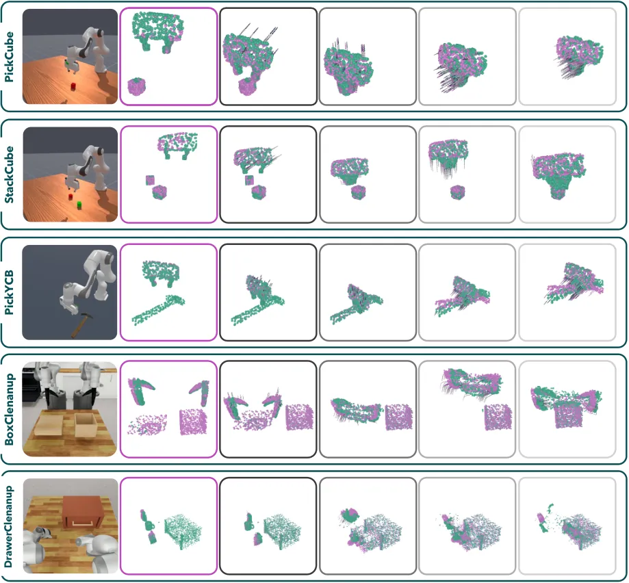
Figure 3: Purple points show the ground-truth trajectory and teal points show the prediction. Each future frame is conditioned on the previous predicted cloud and the recorded action.

Closed-loop and open-loop planning

Planning is evaluated on PickCube, StackCube, and PickYCB. Closed-loop runs execute at most 100 environment steps and use 200 MPPI samples with a rollout horizon of 10 at each step. The comparison separates ground-truth completion, learned completion, PF+, partial 3DPWM, and an analytic forward-kinematics baseline. Ground-truth completion provides an upper bound on what the dynamics model can achieve when perception is not the limiting factor.

Evaluation	PickCube	StackCube	PickYCB
Closed-loop with ground-truth completion	88%	about 78%	about 60%
Closed-loop with learned completion	A 2 to 10 percentage-point drop on the harder settings, depending on task
Open-loop partial-cloud baseline	1/20, or 5%	0%	0%
Novel-task adaptation: MugCleanup	75%	Not applicable	Not applicable
Novel-task adaptation: Coffee	60%	Not applicable	Not applicable
Novel-task adaptation: CoffeePreparation	45%	Not applicable	Not applicable

With perfect completion, the success rate falls from 88% on PickCube to roughly 78% on StackCube and 60% on PickYCB. Learned completion introduces additional errors and lowers harder tasks by 2 to 10 points. This gap is important: the perception stage is accurate enough to support planning, but not solved. The analytic forward-kinematics baseline remains strong on the simpler tasks, because direct geometric approach explains much of their required behavior. Its advantage disappears on the diverse 78-object PickYCB setting, where modeling interaction outcomes becomes more valuable.

The open-loop experiment is a stricter test of whether the model can act like a proxy simulator. The system observes only the initial cloud and plans an entire action sequence without visual correction. PF+ and the partial-cloud variant almost completely fail: PickCube reaches only 1/20 and the other tasks reach zero. The proposed model retains non-trivial success even with learned completion. Its prediction must therefore remain useful over a sequence, not merely reproduce the next frame.

Novel task composition and sim-to-real transfer

The authors train dynamics on the shorter MugCleanup and Coffee tasks, then deploy the resulting model on CoffeePreparation. The longer task requires placing a cup at a coffee machine, retrieving a pod from a drawer, loading it, and closing the lid. Success is 75% on MugCleanup, 60% on Coffee, and 45% on the composed task. PF+ already struggles on the short tasks and fails completely when they are chained. The drop from 60% to 45% quantifies both the promise and the cost of composition: complete geometry supports generalization, while execution and prediction errors still accumulate.

The real-world setup uses a Franka Panda with a parallel jaw, an Intel RealSense D455, and a static third-person view. The camera is extrinsically calibrated to the robot and ManiSkill2 coordinate system. Task-relevant objects are segmented with vision-language prompts and SAM3, then completed by the YCB-fine-tuned model. The best simulated PickYCB checkpoint is deployed without real-world fine-tuning. Planning uses 30 to 50 step open-loop horizons executed in chunks, with 10 trials per method and task.

Success is 60% for PickDrill, 40% for PickApple, and 80% for PlaceApple. PF+ is approximately 0%, 0%, and 70%, respectively. Placement is easier for both systems because the plate offers a broad support region. The difference is concentrated in picking. When only the camera-facing side of an apple or drill is visible, the object centroid and grasp region are underconstrained. Completion gives the dynamics model a more realistic volume, improving its prediction of how the grasp affects the object. Remaining failures are attributed mainly to biased centroid estimates, segmentation errors, and completion errors.

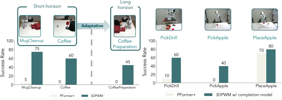
Figure 4: Left, two short tasks are composed into CoffeePreparation. Right, the simulated model transfers to PickApple, PickDrill, and PlaceApple on a real Franka robot.

Training and deployment cost

Training takes 12 to 24 hours on one L40, with larger point sets and higher-dimensional actions approaching the upper end. Planning one action takes about 1.07 seconds on an RTX 4090. The latency comes primarily from sequential point-cloud rollouts, since every future step depends on the previous predicted coordinate. Real tasks execute chunks of 20 planned actions before observing again.

That rate is acceptable for a quasi-static tabletop task and too slow for high-frequency dynamic manipulation. MPPI further multiplies the cost by evaluating many candidates. The authors suggest chunked multi-step prediction with custom CUDA kernels and lower-dimensional action representations, but those are future engineering directions rather than demonstrated speedups.

Ablations

The main design ablations vary the number of register tokens and the training rollout horizon. Lower values are better. PickCube tests short-horizon manipulation, PickYCB tests object diversity, and MugCleanup tests long-horizon interaction with substantial occlusion.

Task	Register tokens			Multi-step loss horizon H
	0	1	2	3	5	10	15
PickCube	0.013	0.009	0.009	0.068	0.038	0.021	0.009
PickYCB	0.052	0.028	0.027	0.161	0.117	0.044	0.028
MugCleanup	0.178	0.022	0.020	0.102	0.036	0.028	0.022

The largest register-token gain comes from zero to one. This supports the proposed role of the dummy key: the problem is not simply insufficient capacity, but the absence of a route through which unrelated points can avoid action information. A second token lowers PickYCB error by 0.001 and MugCleanup by 0.002, so the authors choose one to limit complexity.

Longer multi-step supervision improves every task. For MugCleanup, error drops from 0.102 at horizon 3 to 0.022 at horizon 15. The training objective therefore matches the recursive use of the model at deployment. The result is not merely a longer fit to a single future: the model is repeatedly trained through states produced by its own predictions.

Limitations

Segmentation is the first failure source. SAM3 sometimes misses partially occluded objects or objects held by the gripper. The authors report that 4 of 12 real-world failures come from this stage. If an object is not segmented, the completer receives no input and the world model treats the missing entity as absent. A planner cannot recover that geometry through higher-level reasoning alone.

Completion is the second and more frequent source. The YCB completion data renders each object from 100 random viewpoints on a unit sphere, but each training example contains only that individual object. It lacks scene-level occlusion and does not fully reproduce the noise distribution of a real depth sensor near boundaries and reflective surfaces. Five of 12 real failures are attributed to completion. The component responsible for most of the gain is therefore also the most fragile interface.

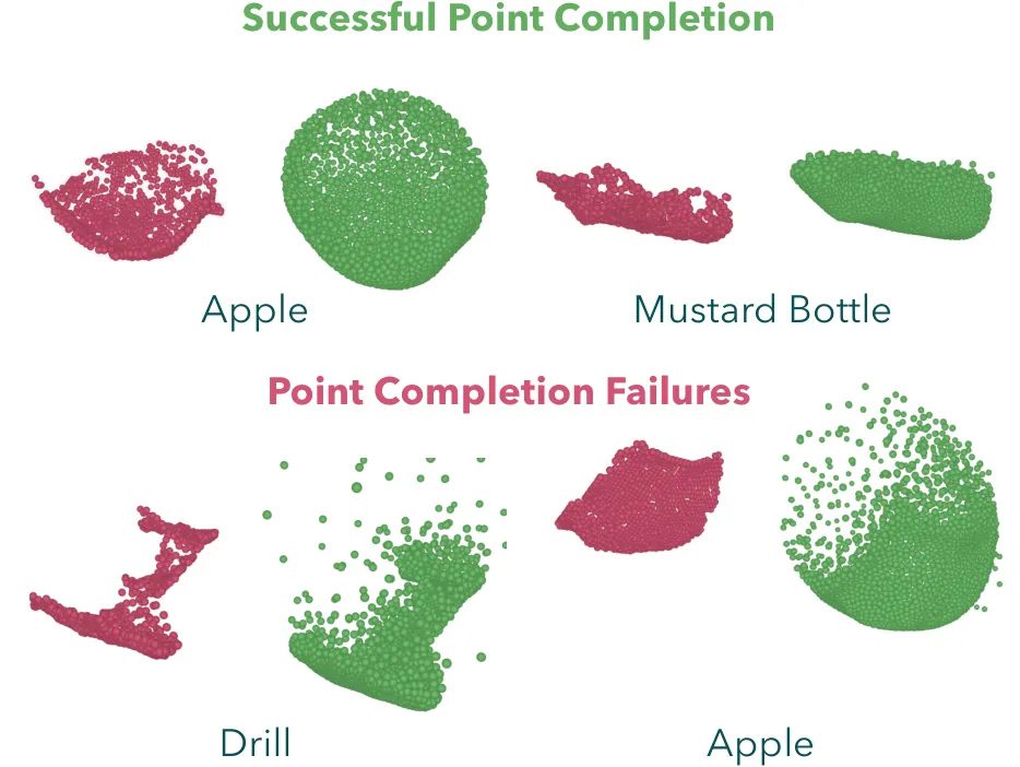
Figure 6: The top row shows successful completions for an apple and a mustard bottle. The bottom row shows failures on a drill and an apple, including shifted volume and out-of-boundary points.

The modular architecture creates cascading risk. The vision-language model, segmentation, depth back-projection, completion, dynamics, and planner are optimized as separate stages. Their interfaces make components replaceable, but a calibration error, poor depth region, incorrect prompt, or completion artifact propagates forward. A small Chamfer change can still move a center of mass enough to alter the ordering of planned actions.

Sequential point rollout also limits speed and task scope. Chunked open-loop planning works for quasi-static tabletop manipulation but is poorly suited to fast dynamics. Contact is not part of the state, and the 2.5-centimeter grasp rule ignores force, friction, and slip. These choices make the method less suitable for throwing, in-hand dexterity, or strongly contact-rich assembly.

Finally, the claim concerns the value of completion, not the claim that completion solves perception. Complete point clouds can be complete yet physically wrong. Transparent, thin, or severely occluded objects remain difficult. The paper shows that completed geometry is a better training and deployment representation than visible partial geometry, but it does not eliminate the need for robust scene-level perception.

Conclusion

The central contribution is a shift in where the hard problem is handled. Instead of asking a dynamics network to infer hidden geometry while learning physics, the system completes task-relevant objects before dynamics prediction. Forward-kinematics points provide the action source, completed object points provide the affected volume, and a task-agnostic point model predicts their joint motion. This representation narrows the gap between mesh-based simulation and single-view deployment.

The experiments support the argument at several levels: six rollout tasks covering two embodiments, closed-loop and open-loop planning, composition into a longer unseen task, and real-world transfer without dynamics fine-tuning. The most promising next steps are scene-level completion data, chunked parallel time prediction, and joint modeling of geometry and contact. Together they address the three bottlenecks that currently keep this approach in relatively slow, quasi-static manipulation.

Golden quote: Complete geometry is not valuable because it makes the future look better; it is valuable because training and deployment can then reason about where an object is and how it will be pushed in the same spatial language.

Further Reading

• arXiv abstract and PDF
• Full paper, version 2 HTML
• Author project page
• Code repository, currently marked as coming soon