Into the LidarVerse: A Real-Time Unified LiDAR World Model Across Tasks and Sensors

Into the LidarVerse: A Real-Time Unified LiDAR World Model Across Tasks and Sensors
Henry Che (NVIDIA / UIUC), Xuanchi Ren (University of Toronto), Sanja Fidler (University of Toronto / NVIDIA), Shenlong Wang (UIUC), Laura Leal-Taixe (NVIDIA), Shengyu Huang (NVIDIA)
arXiv:2610.19201v1 [cs.CV], submitted 2026-10-13 · arXiv:2610.19201 · project page, NVIDIA SIL · code: nv-tlabs/LidarVerse
Code status: public. The repository ships the tokenizer (a NATTEN-based Transformer VAE), the diffusion training and inference stack, the SF-DMD self-forcing distillation trainer, and the three-stage config at diffusion/training/config/text2world_hdmaptolidar/experiment_lidarverse.py; checkpoints are hosted on HuggingFace under nvidia/lidarverse.

In One Line

LidarVerse folds the two rival schools of LiDAR simulation into a single conditional generative model. Reconstruction-based simulators fit a scene representation to a captured log and buy geometric fidelity with hours of per-scene optimization; generative simulators amortize across a dataset but cannot hold a scene together over a long rollout. Here, an attention-only range-image tokenizer builds a latent space shared across sensors, a bidirectional teacher initialized from Cosmos-Transfer2.5-2B learns one interface over four independently switchable conditions (a LiDAR prefix, an HD-map, a persistent spatial cache, and optional text), and self-forcing distribution matching distills it into a four-step block-autoregressive student with a nine-frame rolling K/V cache and a 0.15 m world-aligned voxel cache. The same weights generate new scenes at 11.18 FPS and action-conditioned scenes at 11.30 FPS on one H100, forecast point clouds, and resimulate captured scenes with zero per-scene optimization. What separates the three tasks is not the parameters but how much scene evidence is available at inference time.

1. The Gap: Reconstruction Keeps the Scene, Generation Keeps the Scale

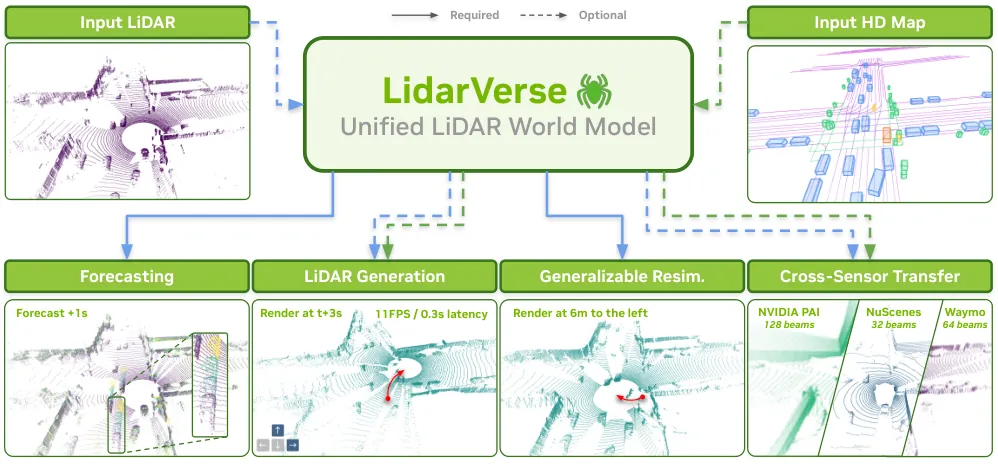
Figure 1 (paper teaser): one distilled causal checkpoint generates new worlds, forecasts future point clouds, or resimulates observed scenes along new sensor trajectories, depending only on which scene evidence is supplied. All three run in real time over long horizons.

The introduction frames the requirement bluntly. Robots and autonomous vehicles have to behave safely over a long tail of environments, trajectories, and interactions that cannot be collected exhaustively, so a sensor simulator needs two capabilities at once: preserving an observed world while changing the sensor trajectory, and creating new worlds beyond recorded experience. NVIDIA Omniverse NuRec stands for the first, OmniDreams for the second. LiDAR sits in an awkward spot in this landscape because it returns direct geometric measurements that survive poor illumination, yet its returns are sparse and strongly viewpoint dependent. Three engineering constraints come on top: the observations must be accurate, they must stay temporally coherent under sensor motion, and the simulator must be fast enough to use interactively.

Neural LiDAR simulation developed along the same divide. Reconstruction-based methods fit an explicit neural scene representation to a captured log and render LiDAR from novel poses. Their persistent 3D representations deliver strong geometric consistency and precise viewpoint control, which is exactly what scene resimulation asks for. The price is that fitting a single scene can take hours, and the resulting simulator is welded to that manually collected log: it can vary the trajectory inside one scene but cannot scale to a diverse distribution of new environments.

Generative methods amortize scene modeling over the dataset and learn a distribution to sample from. Their bottleneck is not the diffusion model but the representation. Operating on unordered point sets is inefficient and forfeits the mature image and video generation stack. Range images preserve the scanning topology and are sensor native, but high-resolution range sequences are expensive to model directly with pixel-space diffusion. Tokenizers built for RGB video match range images poorly, and existing LiDAR tokenizers generally target a single scanning pattern. The consequence is a field of generators that specialize in one sensor configuration, emit short sequences, or need many denoising steps.

LidarVerse reframes the problem: generation, forecasting, and resimulation differ only in how much scene evidence exists at inference. With no observed geometry the model synthesizes new worlds from scene-level conditions; an observed LiDAR prefix turns the same model into a point-cloud forecaster; a persistent spatial cache built from observed sweeps anchors it to one particular world for generalizable resimulation under a new sensor trajectory, with no per-scene optimization. These are three ways of querying one conditional prior, not three architectures.

2. Preliminaries: Range Images and Two Inverse Projections

Everything enters and leaves the model as a range image. A pixel at row $j$, column $i$ carries a range $r_{j,i}$, and the spherical-to-Cartesian mapping is

$$\mathbf{p}_{j,i}=\begin{bmatrix}x_{j,i}\\ y_{j,i}\\ z_{j,i}\end{bmatrix}=r_{j,i}\begin{bmatrix}\cos\phi_{j}\cos\theta_{i}\\ \cos\phi_{j}\sin\theta_{i}\\ \sin\phi_{j}\end{bmatrix}$$

The inverse projection looks up the calibrated row and column angles of each point:

$$\theta_{k}=\operatorname{atan2}(y_{k},x_{k}),\qquad \phi_{k}=\arcsin(z_{k}/r_{k}),\qquad r_{k}=\lVert\mathbf{p}_{k}\rVert_{2}$$

When several points land on the same ray, only the nearest return is kept. Valid ranges are clamped to $[r_{\min},r_{\max}]$ and normalized to $[-1,1]$, and a validity mask $\mathbf{M}\in\{0,1\}^{H\times W}$ separates real measurements from missing returns. The default representation concatenates channels, $\mathbf{I}=[\mathbf{R}\mid\mathbf{M}]$; when intensity is available it is clipped to $[0,255]$, normalized to $[0,1]$, and appended as a third channel. Stacking $T$ ordered sweeps gives $\mathbf{X}=\operatorname{Concat}(\mathbf{I}_{1},\ldots,\mathbf{I}_{T})\in\mathbb{R}^{T\times H\times W\times C_{\mathrm{in}}}$ with $C_{\mathrm{in}}=2$, or $3$ with intensity.

3. A Universal Tokenizer Built on Neighborhood Attention

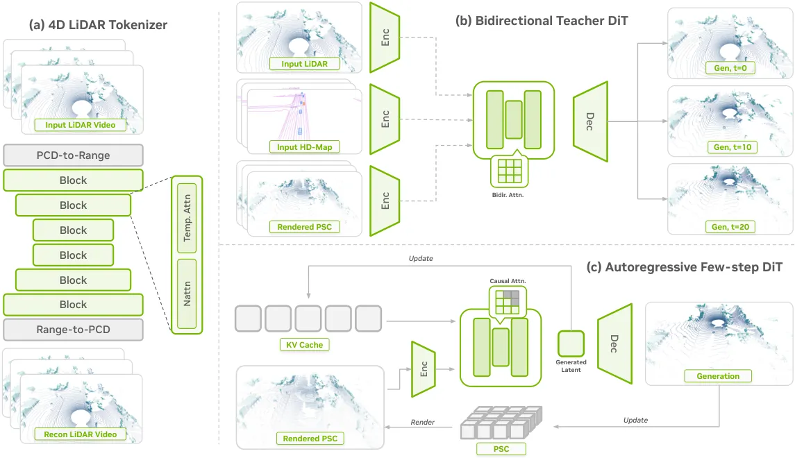
Figure 2 (paper architecture figure): three training stages address representation, task unification, and deployment. (a) A fully attention-based LiDAR tokenizer learns a shared latent space while preserving spatial and temporal structure. (b) A bidirectional teacher learns one interface over a LiDAR prefix, an HD-map, a persistent spatial cache, and optional text. (c) Causal distillation plus a rolling spatial cache make the same interface run in real time over long horizons.

An encoder maps $\mathbf{X}$ to a latent $\mathbf{z}=\mathcal{E}(\mathbf{X})\in\mathbb{R}^{\frac{T}{p_{t}}\times\frac{H}{p_{s}}\times\frac{W}{p_{s}}\times c}$ and a decoder reconstructs $\widehat{\mathbf{X}}=\mathcal{D}(\mathbf{z})$. RGB video tokenizers conventionally use convolutional backbones, and the paper explains why that fails here: angular bins that are neighbors in a range image can correspond to surfaces meters apart in 3D. Fixed convolutional aggregation blurs depth discontinuities, which is precisely the depth bleeding and wavy boundary artifact reported in prior LiDAR generation work.

The replacement is neighborhood attention (NATTEN), which aggregates content-adaptively inside each local window and avoids the quadratic memory of global self-attention. Spatial blocks use a $5\times 35$ window with no dilation and circular padding across the azimuth wrap, following Nakashima et al. Temporal context is injected by interleaving each spatial NATTEN block with temporal self-attention at the two lower-resolution stages, under a causal mask so that each frame depends only on the current and preceding frames. That choice makes the tokenizer compatible with causal and variable-length rollouts before any world model is trained.

Cross-sensor reach comes from two decisions stacking. First, $p_{t}=1$: LiDAR streams run at much lower frame rates than RGB video (Waymo is 10 Hz), so there is little temporal redundancy to compress, and compressing time discards frame-level geometry while binding the latent to one acquisition rate. Second, the fully attention-based backbone aggregates by content rather than by a fixed kernel, so it can absorb different spatial sampling patterns. Together they let a single tokenizer checkpoint adapt across beam layouts, angular resolutions, and frame rates.

Concretely: a symmetric Transformer with channel widths $[128,256,512]$, spatial depths $[4,2,4]$, and $[4,16,16]$ heads, i.e. ten spatial blocks in each of the encoder and decoder; a $2\times 2$ input patch embedding, MLP expansion ratio 3, two latent-mapping layers, and a $c=64$ latent. Spatial compression is $8\times 8$, mapping one $2\times 64\times 1024$ sweep to a $64\times 8\times 128$ latent with temporal resolution intact. The tokenizer has 64.5M parameters and trains for 120k iterations under

$$\mathcal{L}_{\mathrm{tokenizer}}=\lambda_{\mathrm{depth}}\mathcal{L}_{\mathrm{depth}}+\lambda_{\mathrm{point}}\mathcal{L}_{\mathrm{point}}+\lambda_{\mathrm{mask}}\mathcal{L}_{\mathrm{mask}}+\lambda_{\mathrm{KL}}\mathcal{L}_{\mathrm{KL}}$$

where $\mathcal{L}_{\mathrm{depth}}$ is an $\ell_1$ loss on valid reconstructed ranges, $\mathcal{L}_{\mathrm{point}}$ is an $\ell_1$ loss on the valid 3D points recovered from the reconstructed range image through Eq. 1, $\mathcal{L}_{\mathrm{mask}}$ is binary cross-entropy on the reconstructed validity mask, and $\mathcal{L}_{\mathrm{KL}}$ is the KL divergence between the latent posterior and a standard normal prior under reparameterization. The weights are $\lambda_{\mathrm{depth}}=\lambda_{\mathrm{point}}=\lambda_{\mathrm{mask}}=1$ and $\lambda_{\mathrm{KL}}=10^{-6}$. A KL weight that small barely constrains the latent, which tells you the tokenizer is optimized for reconstruction fidelity rather than sampling convenience; sampling is the diffusion model's job.

4. The Bidirectional Teacher and Four Independently Droppable Conditions

The teacher is initialized from Cosmos-Transfer2.5-2B: 28 diffusion transformer blocks, hidden width 2048, 16 attention heads, each block applying spatiotemporal self-attention, text cross-attention when relevant, and an MLP with AdaLN-LoRA time conditioning. The 3D rotary positional embeddings and the flow-matching formulation are retained; only the input and output projections are adapted to the LiDAR latent and conditioning channels. Given a clean latent $\mathbf{z}$, noise $\bm{\epsilon}\sim\mathcal{N}(\mathbf{0},\mathbf{I}_{\mathrm{lat}})$ and a flow time $\tau\in[0,1]$ define

$$\mathbf{z}_{\tau}=(1-\tau)\mathbf{z}+\tau\bm{\epsilon},\qquad \mathbf{v}^{*}=\frac{\partial\mathbf{z}_{\tau}}{\partial\tau}=\bm{\epsilon}-\mathbf{z}$$

and the teacher learns to predict $\mathbf{v}^{*}$. The four conditions encode forms of scene evidence, not task identities.

(1) LiDAR prefix. $K$ observed sweeps become range images, pass through the tokenizer, and their clean latents occupy the first $K$ temporal positions, concatenated in time with the noisy target latents. A binary mask marks observed positions and the generative loss is applied only to target positions. This is what enables continuation from one or more observations.

(2) HD-map and actor layout. The layout condition carries lane centerlines, road markings, road boundaries, crosswalks, and 3D actor boxes. Given static map primitives $\mathcal{M}$, actor boxes $\mathcal{B}_{t}$, and the target LiDAR-to-world pose $\mathbf{T}_{t}$, they are transformed into the target LiDAR frame and rasterized into a range-aligned image

$$\mathbf{H}_{t}=\Pi_{\mathrm{map}}(\mathcal{M},\mathcal{B}_{t};\mathbf{T}_{t})$$

where $\Pi_{\mathrm{map}}$ keeps the nearest element on each calibrated ray using Eq. 2, with preprocessing from the utility released with Cosmos-Drive-Dreams. The result is encoded as $\mathbf{h}_{t}=\mathcal{E}(\mathbf{H}_{t})$ and concatenated channel-wise with the noisy LiDAR latent.

(3) Persistent spatial cache (PSC). A world-aligned geometric memory $\mathcal{G}$ accumulated from observations or from previous generations, projected at the target pose into

$$\mathbf{G}_{t}=\Pi_{\mathrm{geometry}}(\mathcal{G};\mathbf{T}_{t})$$

with $\Pi_{\mathrm{geometry}}$ transforming world-frame points into the target LiDAR frame and keeping the nearest range per calibrated ray. The image is encoded as $\mathbf{g}_{t}=\mathcal{E}(\mathbf{G}_{t})$ and again concatenated channel-wise. During teacher training $\mathcal{G}$ is built from ground-truth sweeps in two modes: static background, which removes points inside labeled dynamic boxes before accumulation, and frozen dynamic, which additionally accumulates each actor in its own local frame and places it according to its box pose at time $t$. The causal model uses the identical projection, encoding, and injection procedure but builds $\mathcal{G}$ online from generated history. That single invariant is what lets the conditioning interface survive all three stages.

(4) Text. Following Cosmos-Drive-Dreams, Qwen2.5-VL-7B-Instruct rewrites scene descriptions into captions with diverse weather and appearance attributes, and the Cosmos-Reason1 text encoder maps each caption to token embeddings that serve as cross-attention context in every block. Text governs environmental appearance while the spatial conditions anchor geometry, so the two never compete for the same job.

In the unified-conditioning stage every factor is sampled independently: with probability 0.5 the prefix length $K$ is drawn uniformly from $\{1,2,4,8,10,12,16\}$ and otherwise $K=0$; the HD-map is dropped with probability 0.5 via a null token; the PSC is sampled as null, static-background, or frozen-dynamic geometry with probabilities $0.1$, $0.45$, and $0.45$, and in frozen-dynamic mode the number of source sweeps $N_{\mathcal{G}}$ is uniform over $\{1,2,4,8,10,12,16,20\}$; text embeddings get 20% classifier-free dropout. This factorized sampling exposes the model to many evidence combinations without task tokens or task objectives.

The curriculum is staged rather than mixed from the start: 270k iterations split into 150k of HD-map-conditioned generation on nine-frame clips, 100k on 21-frame clips, and 20k of unified conditioning on 21-frame clips. The authors report this produced better results than training with joint conditioning directly. Global batch size is 32, AdamW with $\mathrm{lr}=10^{-5}$, $\beta=(0.9,0.999)$, weight decay 0.01, and a rectified-flow timestep shift of 5.

5. Causal Distillation With Self-Forcing Distribution Matching

Full-sequence attention plus iterative denoising makes the teacher unusable for interactive simulation, so it is distilled into a few-step block-autoregressive student. Causal initialization starts from the teacher weights and replaces full temporal attention with a block-causal pattern: a singleton attention sink supports generation from a single frame, followed by four-frame blocks. Clean ground-truth latents from preceding blocks live in a K/V cache while each active block is perturbed and denoised independently. This stage runs 10k teacher-forcing iterations on 21-frame clips purely to adapt the weights to causal attention.

Self-forcing distribution matching distillation (SF-DMD) then takes over. The student samples each four-frame block with four shifted rectified-flow SDE steps, commits the generated clean latents to its K/V cache, and updates the recurrent conditioning state before sampling the next block. Training therefore consumes exactly the self-generated temporal and geometric history that inference will produce, which is the point of self-forcing. The objective is not to regress the rollout onto a paired ground-truth sequence but to match its distribution to the real LiDAR latent distribution. Let $\widetilde{\mathbf{z}}$ be a self-rolled-out latent sequence, perturbed to $\widetilde{\mathbf{z}}_{\tau}$; a frozen real-data denoiser and a learned generated-data denoiser produce clean estimates $\widehat{\mathbf{z}}_{0}^{\mathrm{real}}$ and $\widehat{\mathbf{z}}_{0}^{\mathrm{gen}}$. For a replayed denoising step the adaptive scale is $a=\operatorname{mean}\lvert\widetilde{\mathbf{z}}-\widehat{\mathbf{z}}_{0}^{\mathrm{real}}\rvert+\varepsilon$, and the student's clean prediction $\widehat{\mathbf{z}}_{0}^{\mathrm{stu}}$ is optimized by

$$\mathcal{L}_{\mathrm{SF\text{-}DMD}}=\mathbb{E}\!\left[\frac{1}{2}\left\|\widehat{\mathbf{z}}_{0}^{\mathrm{stu}}-\operatorname{sg}\!\left[\widetilde{\mathbf{z}}-\frac{\widehat{\mathbf{z}}_{0}^{\mathrm{gen}}-\widehat{\mathbf{z}}_{0}^{\mathrm{real}}}{a}\right]\right\|_{2}^{2}\right]$$

with $\operatorname{sg}$ the stop-gradient and $a$ normalizing the update adaptively. The real-data denoiser stays frozen; the generated-data denoiser is initialized from it and continues training with the rectified-flow objective on self-rollouts. The stage lasts only 2k iterations, updating the fake-score network every cycle and the student every five cycles, with student $\mathrm{lr}=2\times10^{-6}$, fake-score $\mathrm{lr}=4\times10^{-7}$, distillation teacher CFG 3.0, and a four-step SDE ladder $(1,\,15/16,\,5/6,\,5/8,\,0)$ at $\eta=1$ where zero is the clean endpoint. The finished student keeps a nine-frame rolling K/V cache including one persistent sink frame.

6. The Rolling Persistent Spatial Cache

A finite temporal K/V cache holds only recent latent context, and lengthening it costs memory and compute at every step. Once an observation leaves that window the model can lose scene structure it generated earlier. The fix is a sparse world-aligned voxel map $\mathcal{V}$ used as a rolling PSC: the conditioning interface is unchanged from Section 3.2, but the underlying geometry is constructed online from generated history. After block $b$ is generated, each latent $\widetilde{\mathbf{z}}_{t}$ is decoded into a point cloud $\widetilde{\mathcal{X}}_{t}$, registered to the common world frame with its sensor pose, and folded into the map:

$$\mathcal{V}_{b}=\mathcal{U}(\mathcal{V}_{b-1},\mathcal{Y}_{b}),\qquad \mathcal{Y}_{b}=\bigcup_{t\in\mathcal{T}_{b}}\mathbf{T}_{t}\widetilde{\mathcal{X}}_{t}$$

Each occupied voxel $v$ stores its most recently registered point $\mathbf{p}(v)$, an observation count $n^{\mathrm{obs}}(v)$, and a removal count $n^{\mathrm{rem}}(v)$, with each source frame contributing at most one observation per voxel. An observation updates the point, increments the count, and resets the removal counter; valid free-space evidence contradicting the voxel increments the removal counter instead. Requiring repeated observations keeps transient generation errors out of persistent memory, and requiring repeated contradictions stops one inconsistent sweep from deleting valid structure. Before block $b+1$ is generated, only confirmed and unremoved voxels are kept and rendered at each requested target pose:

$$\mathcal{P}(\mathcal{V}_{b})=\left\{\mathbf{p}(v)\mid n^{\mathrm{obs}}(v)\geq N_{\min},\; n^{\mathrm{rem}}(v)<N_{\mathrm{rem}}\right\}$$

$$\mathbf{g}_{t}^{\mathrm{cache}}=\mathcal{E}\!\left(\Pi_{\mathrm{geometry}}(\mathcal{P}(\mathcal{V}_{b});\mathbf{T}_{t})\right),\qquad t\in\mathcal{T}_{b+1}$$

The implementation paragraph is unusually specific: $0.15\,\mathrm{m}$ cubic voxels; stale geometry is detected by projecting eligible cached points into the last sweep's range image and incrementing the removal counter when the surrounding $3\times3$ pixels contain valid returns farther than $0.75\,\mathrm{m}$; only voxels with $n^{\mathrm{obs}}\geq N_{\min}=3$ contribute to the rendered PSC; voxels reaching $N_{\mathrm{rem}}=2$ contradictions are deleted together with their counters and must re-earn the observation threshold if seen again. Cache updates happen only after block generation, so a block can only ever query geometry produced by earlier blocks. No self-conditioning, no future leakage.

flowchart TB
    RI[Range image 2x64x1024
range R plus validity mask M] --> TOK[Universal tokenizer
spatial NATTEN 5x35 circular azimuth
causal temporal attention pt=1]
    TOK --> LAT[Shared latent 64x8x128
c=64 and 64.5M params]
    LAT --> TEA[Bidirectional teacher 28 blocks 2048 wide
Cosmos-Transfer2.5-2B init
flow matching predicts v]
    PRE[Condition 1 LiDAR prefix K frames
p=0.5 with K in 1 2 4 8 10 12 16] --> TEA
    MAP[Condition 2 HD map and actor boxes
H_t concatenated channel wise and dropped 0.5] --> TEA
    PSC[Condition 3 persistent spatial cache G_t
null 0.1 static background 0.45 frozen dynamic 0.45] --> TEA
    TXT[Condition 4 text caption
Qwen2.5-VL rewrite with CFG dropout 20 percent] --> TEA
    TEA -->|curriculum 150k then 100k then 20k| INIT[Causal initialization 10k iters
one sink frame plus four frame blocks
teacher forcing]
    INIT -->|SF-DMD 2k iters
student updated every 5 cycles| STU[Four step causal student
SDE ladder 1 15/16 5/6 5/8 0
nine frame rolling K/V cache]
    STU -->|decode and register each block| ROLL[Rolling voxel map 0.15 m
update operator U over V_b and Y_b
N_min=3 and N_rem=2 and 0.75 m staleness]
    ROLL -->|re-enter only after the block| STU
    STU --> OUT[One checkpoint on one H100 at 11 FPS]
    OUT --> G1[No observed evidence becomes generation]
    OUT --> G2[Prefix becomes point cloud forecasting]
    OUT --> G3[PSC becomes resimulation with zero per scene optimization]

Diagram: the three-stage pipeline and the inference-time evidence spectrum. The feedback edge from the rolling voxel map is the interesting one. The student writes its own outputs into the map and reads them back as conditioning for the next block, always one block behind.

Inference therefore forms a continuum. Every mode receives the requested target sensor poses, and an HD-map may additionally constrain layout. Adding observed LiDAR evidence, first a prefix and then a PSC, walks the same causal checkpoint from generating a new world, to forecasting an observed sequence, to resimulating a specific captured scene. In resimulation the sparse observed sweeps are accumulated into a fixed frozen-dynamic PSC and rendered at novel poses, with no HD-map condition and no per-scene optimization; in generation the PSC is rolling and built from generated sweeps; in action-conditioned generation user-provided ego actions determine the future sensor poses.

7. Code Correspondences: Every Constant in the Paper Has a Config Key

Correspondence 1: circular NATTEN is literally a circular pad on the azimuth axis. The paper's "$5\times35$ neighborhood window with no dilation and circular padding" appears in tokenizer/networks/transformers/transformer_vae.py as pad/trim around the attention call plus NATTEN's 2D kernel:

def before_attn(self, q, k, v):
    if not self.circular:
        return q, k, v
    padding = self.kernel_size[1] // 2
    q = F.pad(q, (0, 0, 0, 0, padding, padding), mode="circular")
    k = F.pad(k, (0, 0, 0, 0, padding, padding), mode="circular")
    v = F.pad(v, (0, 0, 0, 0, padding, padding), mode="circular")
    return q, k, v

# inside residual()
h = natten.functional.na2d(
    query=q, key=k, value=v,
    kernel_size=self.kernel_size,
    dilation=self.dilation,
    scale=1.0,
    **self._inference_natten_kwargs,
)

The inline comment states the intent directly: # periodic: it is circularly padded before the neighborhood attention, and with circular=False NATTEN clamps the neighborhood at the width edges instead. On the teacher side, diffusion/training/networks/neighborhood_attn.py flips NATTEN's performance switches (use_kv_parallelism_in_fused_na(True), set_memory_usage_preference("unrestricted")) and derives an adaptive configuration from window_size / stride / dilation / is_causal. The paper's claim about avoiding quadratic attention memory is carried by these fused kernels.

Correspondence 2: the PSC numbers are stage-3 config entries. The $0.15\,\mathrm{m}$ voxels, $3\times3$ neighborhood, $0.75\,\mathrm{m}$ staleness margin, $N_{\min}=3$, $N_{\mathrm{rem}}=2$, nine-frame K/V cache, single sink frame, four steps, and $\eta=1$ all show up verbatim in diffusion/training/config/text2world_hdmaptolidar/experiment_lidarverse.py:

stage3_config["model"].update(
    sfdmd_num_steps=4,
    sfdmd_sde_eta=1.0,
    sfdmd_kv_cache_frames=9,
    sfdmd_kv_sink_frames=1,
    sfdmd_tbptt_blocks=2,
    sfdmd_fake_updates_per_cycle=1,
    sfdmd_student_update_freq=5,
    sfdmd_spatial_map_radius_m=100.0,
    sfdmd_spatial_map_voxel_m=0.15,
    sfdmd_spatial_map_voxel_policy="persistent_static",
    sfdmd_spatial_map_observation_unit="block",
    sfdmd_spatial_map_static_min_observations=3,
    sfdmd_spatial_map_free_space_clear=True,
    sfdmd_spatial_map_free_space_margin_m=0.75,
    sfdmd_spatial_map_free_space_misses_to_remove=2,
)

The cache itself is TorchSpatialPointMap in diffusion/training/datasets/lidar_dataset/forecast_warp.py, and its docstring is more explicit than the paper about the promotion rule: a voxel is promoted "only after it is occupied in enough selected observation units", where the block unit counts at most once per committed block; the newest sweep can stay as an ephemeral layer so current dynamic objects remain visible without leaving trails; free-space clearing removes a confirmed voxel "only after repeated in-range current rays pass through it to farther returns", treating nearer returns, missing rays, and out-of-range voxels as unobservable; rendering queries a GPU-resident coarse XY cell index, applies an exact target-local radius mask to that temporary subset, and leaves the global map untouched. The paper's sentence "each source frame contributes at most one observation to a voxel" is the observation_unit="block" setting.

Correspondence 3: the adaptive scale and the four-step ladder are explicit functions. In diffusion/training/utils/sf_dmd.py, fixed_sde_sigmas(num_steps=4, shift=5.0) returns exactly [1.0, 15/16, 5/6, 5/8, 0.0] under a comment reading "Preserve the original four-step schedule exactly for existing runs", and dmd_pseudo_target builds the pseudo-target of Eq. 7:

weight = 1.0 / ((generated.detach() - teacher_x0.detach())
                .abs().mean(dim=reduce_dims, keepdim=True) + eps)
vsd_grad = fake_x0.detach() - teacher_x0.detach()
target = generated.detach() - weight * vsd_grad
return target.detach(), weight.detach()

Here weight is $1/a$ with $a$ the mean absolute difference between generated and teacher_x0 plus $\varepsilon$, vsd_grad is $\widehat{\mathbf{z}}_{0}^{\mathrm{gen}}-\widehat{\mathbf{z}}_{0}^{\mathrm{real}}$, and the outer detach is the $\operatorname{sg}[\cdot]$. The companion sde_renoise implements the $\eta$ blend as eps_used = (1-eta)*eps_implied + eta*eps_fresh followed by (1-sigma)*x0 + sigma*eps_used, and rf_velocity_to_x0 converts the repository's velocity convention into a clean $\mathbf{x}_0$ with a single subtraction.

8. Experiments: Three Protocols, One Set of Weights

Main training and evaluation use the Waymo Open Dataset: 798 training and 202 validation sequences of roughly 20 seconds at 10 Hz, about 160K sweeps, 4.4 hours of sensor data, and 142.8K overlapping 21-frame training clips. The cross-sensor experiments additionally fine-tune the tokenizer and teacher on NVIDIA PAI (111,988 sequences), Waymo, and nuScenes (722 sequences), roughly 640K unique 21-frame clips, sampled with equal probability per dataset so the much larger PAI corpus does not dominate.

8.1 Tokenizer: geometry wins decisively, distribution metrics do not

All baselines are retrained from scratch on the same range-image representation and paired with the same DiT architecture, training recipe, and evaluation protocol on nine-frame sequences, which isolates the latent representation from backbone differences.

Method	ST comp. rate	CD ↓	$L_1$ ↓	AbsRel ↓	JSD ↓	MMD ↓	FUD ↓	ICP Avg ↓	TFLOPs/frame ↓
256x spatiotemporal compression
Cosmos CV	8x8x4	0.439	0.790	0.031	0.061	6.41	46.26	0.089	0.058
Wan2.1	8x8x4	0.297	0.395	0.017	0.057	5.72	37.52	0.077	0.911
Ours	16x16x1	0.175	0.143	0.008	0.061	6.87	32.84	0.072	0.400
32x / 64x compression
LiDM	4x8x1	0.297	0.371	0.016	0.057	5.48	36.22	0.088	0.212
Cosmos LiDARGen	8x8x1	0.384	0.609	0.025	0.062	7.99	85.37	0.085	0.302
Ours	8x8x1	0.115	0.072	0.005	0.065	9.14	18.17	0.059	0.250

Table 1 (condensed from the paper's Table 2): tokenizer comparison under the same DiT. MMD values are multiplied by $10^5$.

Reconstruction is where the design pays off. At $8\times8\times1$ the Chamfer distance is 0.115 against LiDM's 0.297 (61% lower), $L_1$ is 0.072 against 0.371, AbsRel 0.005 against 0.016, and this is against a baseline using a lower 32x compression rate; perceptual FUD is 18.17 against 36.22, a 50% reduction. Forced to the matched 256x regime, the temporally uncompressed design still cuts CD by 41% and AbsRel by 53% while spending 0.400 TFLOPs/frame against Wan2.1's 0.911. Read the distribution columns honestly, though: JSD (0.065 versus LiDM's 0.057) and MMD (9.14 versus 5.48) are not the best in the low-compression regime. BEV statistics and single-frame geometric or feature-space quality are not the same measurement here, and the paper's claim is built on the latter.

8.2 Autoregressive generation: four steps against 256, two orders of magnitude in frame rate

Method	Sampling steps	JSD ↓	MMD ↓	FUD ↓	CTC@1 ↓	CTC@4 ↓	ICP Avg ↓	FPS ↑
HD-map-conditioned generation
LiDARCrafter	256	0.065	14.13	97.24	0.278	0.519	0.120	0.127
LaGen*	35	0.075	19.19	50.29	0.205	0.390	0.071	0.402
Sensor2Sensor*	35	0.047	5.210	37.96	0.225	0.404	0.081	0.421
Ours (causal)	4	0.046	4.390	25.01	0.210	0.331	0.068	11.18
Interactive action-conditioned generation (one ground-truth frame, then 128 generated frames, no HD-map)
LiDARCrafter	256	0.137	54.383	70.38	0.258	0.483	0.104	0.135
LaGen*	35	0.064	12.51	42.31	0.256	0.550	0.074	0.754
Ours (causal)	4	0.054	7.391	24.17	0.213	0.347	0.068	11.30

Table 2 (condensed from the paper's Table 3): MMD values are multiplied by $10^5$; * marks a reimplementation on the authors' tokenizer with a matched DiT, because LaGen and Sensor2Sensor had no public code at the time. Sensor2Sensor has no native mechanism for injecting ego poses and is therefore omitted from the action-conditioned block.

The speed comparison is the one that matters. LiDARCrafter samples 256 steps for FUD 97.24 at 0.127 FPS; LidarVerse samples four steps for FUD 25.01 at 11.18 FPS. Roughly 88x the throughput arrives together with a 3.9x better FUD, so few-step sampling was not paid for with quality. Short-horizon temporal consistency is a mixed bag (CTC@1 0.210 against LaGen*'s 0.205), but the long-offset CTC@4 of 0.331 is the best in the table, which is what causal distillation plus a rolling cache is supposed to buy. The windowed FUD curves in the paper's Figure 9 degrade far more slowly than the baselines, which visibly collapse past 100 frames.

8.3 Point-cloud forecasting: no prediction head, just more evidence

The protocol follows Khurana et al.: three seconds of history predict three seconds of future, i.e. 30 frames in and 30 out at 10 Hz, reported as $L_1$, AbsRel, and inner Chamfer distance at the one, two, and three second marks. One detail is worth flagging: for this task the authors raise the K/V cache from nine frames to 21, because forecasting empirically benefits from longer context. Cache length is a task-dependent knob, not a global constant.

Method	$L_1$ @1s ↓	$L_1$ @3s ↓	AbsRel agg. ↓	CD @1s ↓	CD @3s ↓	CD agg. ↓
Raycasting	2.461	3.768	0.193	1.584	6.049	2.739
4D-Occ	2.146	3.052	0.126	2.173	4.575	2.924
UnO*	2.040	2.654	0.126	1.000	1.440	1.070
Ours	1.482	2.554	0.108	0.485	1.328	0.676

Table 3 (condensed from the paper's Table 4): * marks a best-effort reimplementation, since UnO has no public code. Aggregate columns combine the 1s, 2s, and 3s horizons.

Aggregate Chamfer distance of 0.676 against UnO*'s 1.070 is a 37% improvement, and at the one second mark the gap is 0.485 against 1.000. Qualitatively the model preserves the shapes of traffic participants while producing plausible future motion, and where the future viewpoint reveals regions absent from the input history, naive raycasting fails outright while the shared generative prior completes plausible scene structure. Forecasting here really is an intermediate inference regime of one world model rather than a separate prediction architecture.

8.4 Generalizable resimulation: zero optimization against 76 to 90 minutes

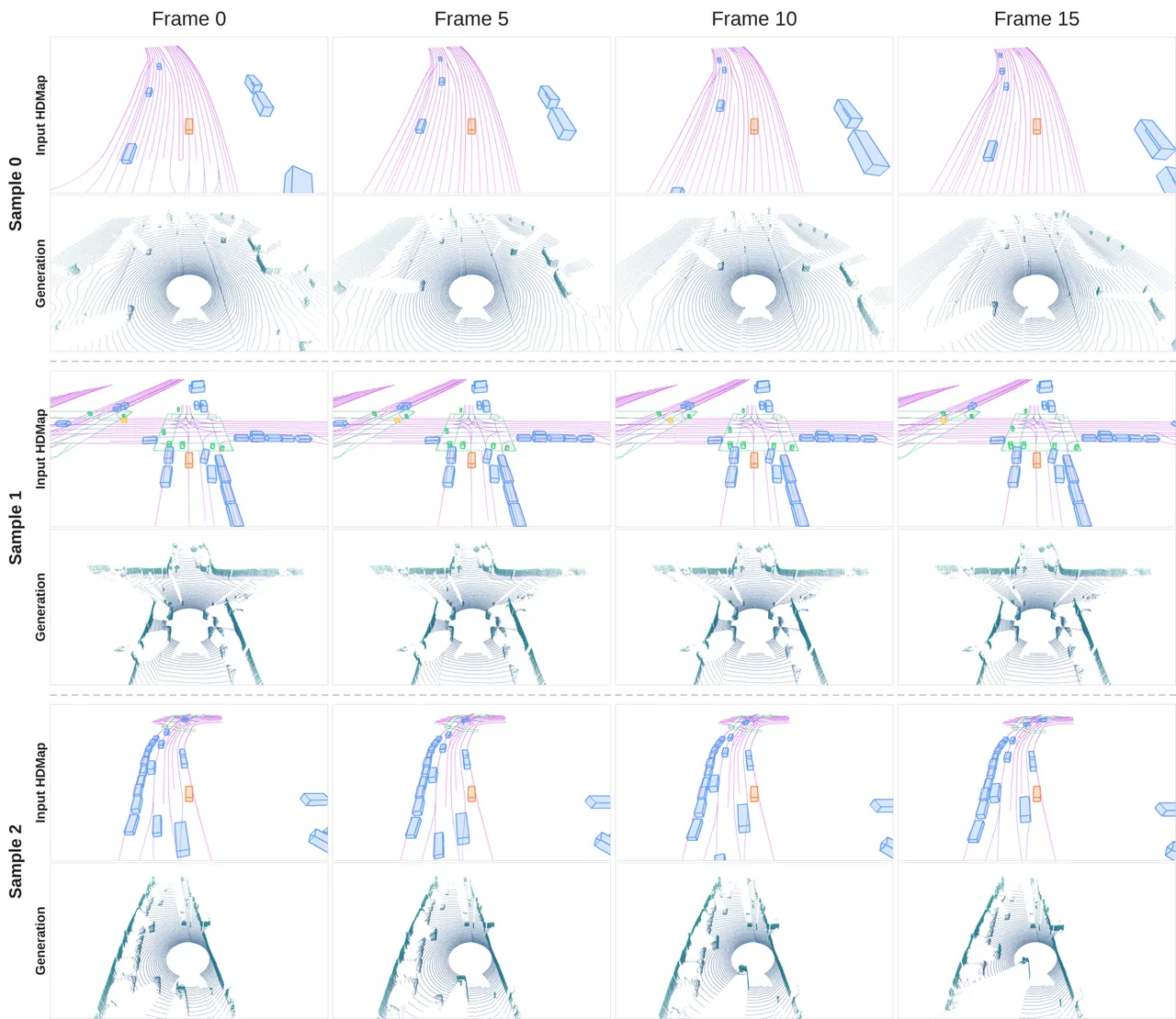
Figure 3 (paper Figure 4): HD-map-conditioned generation from the bidirectional teacher, 21 frames conditioned on the matching 21-frame map sequence. Sample 0 is a highway, Sample 1 a pedestrian-rich intersection, Sample 2 a truck closing from behind. The HD-map is the only condition in each case.

Protocol: non-overlapping 20-frame chunks with frames 0, 4, 9, and 14 as input, leaving 11 interpolation frames (0 to 14 minus the four inputs) and five extrapolation frames (15 to 19). Besides the full 202-sequence validation split, the authors rank sequences by total ego path length, keep the 20 longest, and split each into nine non-overlapping 20-frame windows for a 180-window long-travel subset.

Method	All-202 interp. $L_1$ ↓	All-202 extrap. $L_1$ ↓	All-202 agg. $L_1$/CD ↓	Top-20 agg. $L_1$/CD ↓	Per-scene optim. ↓	Real-time render
LiDAR4D	1.129	1.881	1.364 / 0.273	2.401 / 1.239	89.8 min	No
LiDAR-RT	1.089	1.593	1.247 / 0.256	2.277 / 0.709	76.3 min	Yes
SplatAD	1.799	2.325	1.964 / 0.309	3.603 / 0.542	15.0 min	Yes
Ours (bidirectional teacher)	1.124	1.376	1.202 / 0.200	1.536 / 0.237	0.00	No
Ours (causal student)	1.279	1.682	1.405 / 0.285	1.787 / 0.294	0.00	Yes

Table 4 (paper Table 6): baselines use their released codebases and optimize a separate scene representation per test sequence; LidarVerse uses one checkpoint across all scenes with no test-time optimization. The bidirectional teacher is listed as a quality reference.

This table has to be read in two halves. On the full 202-sequence cohort the causal student's aggregate $L_1$ of 1.405 and CD of 0.285 are worse than LiDAR-RT (1.247 / 0.256) and LiDAR4D (1.364 / 0.273). What it buys is optimization time collapsing from 76 to 90 minutes down to zero, with real-time rendering. The clean sweep is on the long-travel subset: 1.787 / 0.294 against LiDAR-RT's 2.277 / 0.709, LiDAR4D's 2.401 / 1.239, and SplatAD's 3.603 / 0.542, winning every metric with a Chamfer gap above 2.4x. The pattern makes sense. The farther a vehicle travels, the more a per-scene reconstruction has to extrapolate into regions the input sweeps barely touched or never saw, and completing plausible structure is exactly what a generative prior is good at. The bidirectional teacher is the quality ceiling on nearly every metric (1.202 / 0.200 aggregate on All-202) but is explicitly not a real-time renderer.

8.5 Intensity, cross-sensor reach, and ablations

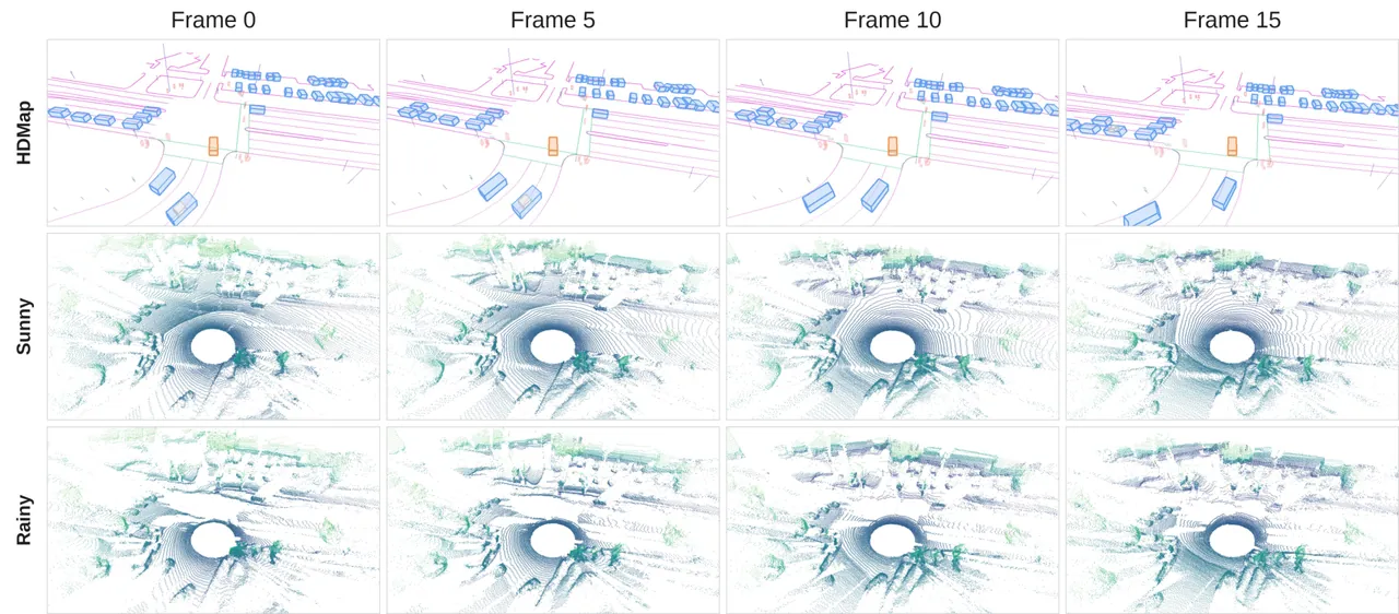
Figure 4 (paper Figure 7): text-controlled weather generation. Rewriting the original sunny prompt to request rain yields a rainy version of the same scene on the NVIDIA PAI data, from the text-conditioned fine-tuned bidirectional teacher. Text handles appearance, spatial conditions handle geometry.

Intensity is added by fine-tuning the tokenizer to reconstruct intensity and then fine-tuning the bidirectional teacher on the combined range-intensity latent. On the top-20 travel-distance subset the intensity RMSE is 0.078 interpolation, 0.091 extrapolation, 0.082 aggregate, level with LiDAR4D (0.077 / 0.094 / 0.082) and clearly ahead of SplatAD (0.115 / 0.134 / 0.121). The cross-sensor result is the counterintuitive one: joint training beats the specialists. The universal tokenizer reaches $L_1$ of 0.065 / 0.037 / 0.087 on nuScenes / Waymo / NVIDIA PAI where single-dataset specialists get 0.087 / 0.056 / 0.286, and on Chamfer distance it wins on Waymo (0.710 versus 0.718) and PAI (1.135 versus 1.240) while conceding slightly on nuScenes (0.568 versus 0.557). It also generalizes to the PandaSet scanning pattern that never appears in training, and swapping the sensor embedding makes one Waymo HD-map produce three distinct scanning patterns.

Four ablations pin the design down. (i) Attention versus convolution at the same $8\times8\times1$ rate, latent dimensionality, DiT, and protocol: $L_1$ 0.072 versus 0.297, CD 0.115 versus 0.278, AbsRel 0.005 versus 0.015, FUD 18.17 versus 26.54, CTC@4 0.339 versus 0.341, TTCE@4 2.463 versus 2.496, and 0.250 versus 0.575 TFLOPs/frame. Better on everything with 57% less tokenizer compute, and both backbones are trained on nine-frame sequences but evaluated on 129-frame sequences from 202 validation clips, where the attention backbone stays more stable beyond its training horizon. (ii) Cache configuration: sweeping the temporal K/V cache over $\{5,9,13,17,21\}$ with the PSC either enabled or replaced by the learned null condition shows that removing the spatial cache substantially worsens temporal consistency while barely touching FUD, and that lengthening the K/V cache improves temporal consistency but costs throughput and fidelity. Hence nine frames plus the spatial cache, with steady-state throughput measured on ten matched clips on one H100. (iii) Voxel confirmation: over $N_{\min}\in\{1,2,3,4,5\}$, registering the latest generated sweep directly ($N_{\min}=1$) gives the best temporal-consistency numbers but worse fidelity, so three is chosen. (iv) Unified versus specialists at matched budget: the unified model improves generation MMD (6.843 versus 6.950) and ICP Avg (0.044 versus 0.047), while two separately trained specialists get better FUD (14.67 versus 16.05) and better resimulation $L_1$/CD (1.380/0.235 versus 1.536/0.237). One checkpoint covers both paradigms at a modest, quantified cost.

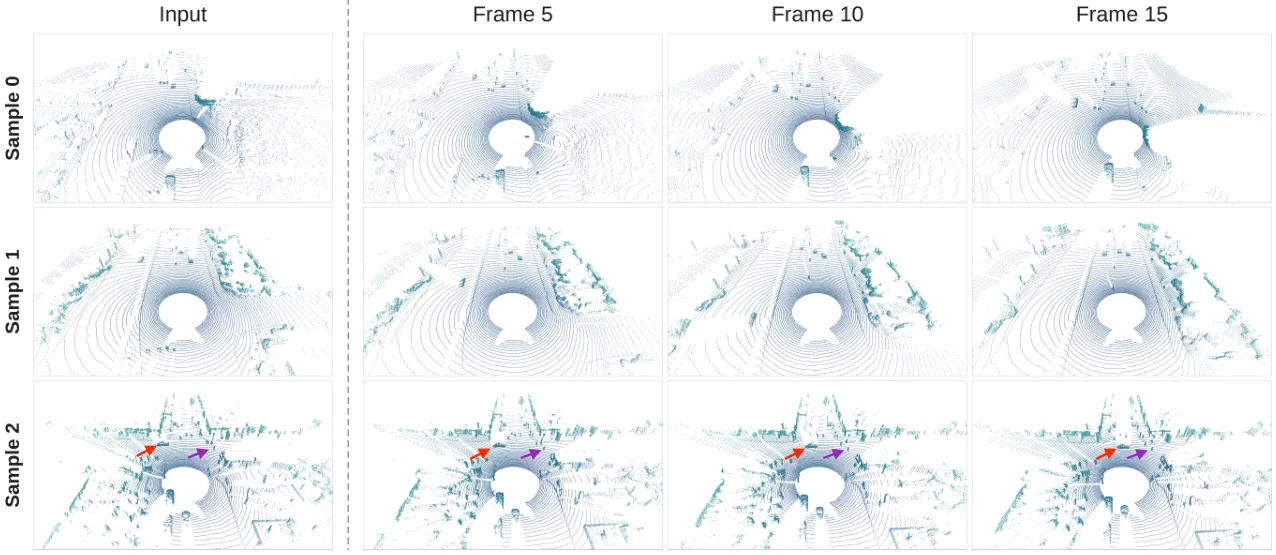
Figure 5 (paper Figure 6): first-frame-conditioned generation from the bidirectional teacher. The red arrow marks a vehicle crossing the intersection and the purple arrow a pedestrian in the crosswalk; Sample 0 is a highway, Sample 1 urban traffic, Sample 2 a crowded intersection. One observed frame, and the rest of the dynamics are produced by the model.

9. Limitations

Four stated by the authors. First, LidarVerse models a single spinning LiDAR; solid-state sensors and joint generation for multi-LiDAR rigs are future work, for which Waymo and Argoverse 2 supply the data. Second, dynamic resimulation depends on annotated object poses during both training and inference, because the frozen-dynamic mode places each actor by its box pose, which caps scalability to unlabeled scenes; annotation-free generalizable resimulation remains an open problem on the LiDAR side. Third, the model is LiDAR only, whereas jointly generating synchronized camera and LiDAR observations is what fuller driving simulation needs. Fourth, the conclusion concedes that no complete closed-loop system is evaluated: interactive action conditioning and requested-pose resimulation are prerequisites for closed loop, not a demonstration of it.

Four more after reading the tables. (1) LaGen*, Sensor2Sensor*, and UnO* are author reimplementations, since those methods had no public code when the experiments ran. Reimplementation strength cannot be checked externally, so those margins deserve a discount; LiDARCrafter and the three resimulation baselines use released codebases and are the firmer comparisons. (2) Real-time belongs to the causal student only. The intensity results, the cross-sensor generation results, and the text-controlled weather example all come from fine-tuned bidirectional teachers, which the paper itself marks as non-real-time in the resimulation table. Counting those capabilities under the same headline model is fine as a capability statement, but they currently run in a different gear. (3) The resimulation win depends on the subset: the causal student trails LiDAR-RT and LiDAR4D on $L_1$ and CD across the full 202 sequences and wins across the board only on the long-travel subset, which happens to be where per-scene reconstruction is weakest. The claim holds, but it is not "better in every setting". (4) The main protocols are Waymo-centric, with PAI and nuScenes appearing only in the cross-sensor study, and there is no planner-in-the-loop metric anywhere, so this is strictly a sensor simulator and not yet a world model you can evaluate a policy inside.

10. Takeaways

The contribution decomposes into three layers that lean on each other. Representation: an attention-only tokenizer that refuses to compress time and uses circular neighborhood attention spatially, so 32-, 64-, and 128-beam sensors share one checkpoint and the latent becomes substantially easier for a downstream diffusion model to fit, with FUD halved and tokenizer compute down 57%. Interface: four conditions that can each be dropped independently, trained with factorized sampling instead of task tokens, so one bidirectional teacher expresses generation, forecasting, and resimulation. Deployment: causal initialization plus SF-DMD compresses it to four block-autoregressive steps, and a rolling voxel cache supplies the persistent geometry a finite K/V window cannot, which together clear the native 10 Hz LiDAR rate on a single H100.

Three things are directly reusable if you build robot or driving simulation. First, if you already work in range images, replacing a convolutional backbone with circular neighborhood attention is close to free: more accurate, cheaper, and more stable past the training horizon. Second, long-horizon consistency does not have to be bought with a longer attention window. Moving memory into an explicit world-aligned voxel map, with a conservative rule that requires repeated observations to promote a voxel and repeated contradictions to delete one, beats simply growing the K/V cache on both quality and throughput. Third, task unification is achievable but priced: the unified model really is behind budget-matched specialists on FUD and resimulation $L_1$, and what you get in return is half the deployment surface. The obvious next steps are the authors' three (solid-state and multi-LiDAR, annotation-free dynamic resimulation, joint camera and LiDAR generation) plus the one the paper does not attempt: putting a planner inside this 11 FPS loop and seeing whether it can actually evaluate a policy.

Golden Lines

"Generation, forecasting, and resimulation are therefore different ways of querying the same learned world, distinguished by the available evidence rather than by model parameters."

"Changing the conditions, rather than the architecture, moves one model between generative simulation and reconstruction-grounded resimulation."