QwenGyre: An Elastic Reinforcement Learning Framework for Training xLong-Horizon Agents

Paper: QwenGyre: An Elastic Reinforcement Learning Framework for Training xLong-Horizon Agents (arXiv:2609.33848, arxiv.org/abs/2609.33848, submitted 2026-09-27, cs.LG / cs.DC)
Authors: Weiqi Wang*, Yuxin Zhou*, Mouxiang Chen*, Siyuan Zhang, Yi Zhang, Yuyan Luo, Zhiyu Yin, Chencan Wu, Jiemin Jiang, Wentao Yao, Chujie Zheng, JianWei Zhang† (Alibaba Token Hub, Alibaba Group; University of Science and Technology of China; Tsinghua University; * equal contribution, † corresponding author)
Code: no public repository is provided with the paper (at the time of checking, GitHub returns zero repositories named QwenGyre). The training and rollout backends are Megatron and SGLang respectively, weight transport reuses the Mooncake Transfer Engine, and the harness is an unmodified Claude Code 2.1.220.

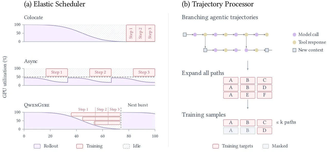
Figure 1: the two challenges QwenGyre targets. (a) The elastic scheduler hands idle rollout capacity to training while in-flight executions keep being served. (b) The trajectory processor rebuilds a branching execution into bounded training samples and counts a repeated target on a shared prefix only once.

In One Sentence

QwenGyre decouples three lifecycles, namely the lifecycle of a harness execution, the lifecycle of a GPU role and the lifecycle of a training sample: an elastic scheduler moves GPUs between rollout and training according to outstanding rollout work without interrupting in-flight executions, while a trajectory processor rebuilds the branching histories produced by a black-box harness into trajectory trees, scores partial progress after a timeout, and extracts bounded trajectories by role priority. On 700K-token rollouts this trains Qwen 3.8 2.4T from 52.5% to 58.5% on NL2RepoBench and delivers up to 1.85× and 1.78× end-to-end speedups over Colocate and Async.

Background and Motivation

LLM agents are taking over progressively longer software engineering tasks. Issue-resolution work such as SWE-bench and its successors only needs to locate a single fix inside an existing repository, and its horizon is a few dozen interactions. Repository generation, system rewrites and whole-codebase refactors push a single execution into a regime of hours, hundreds of model-environment interactions and roughly one million tokens processed across the lifetime. The authors call this regime xLong-horizon: the lifetime token count accumulates the repeated context of every request and can exceed the context limit of any single request.

At that scale online reinforcement learning hits a scheduling wall first. A Colocate design makes one group of GPUs switch wholesale between rollout and training; under xLong the rollout distribution has a severe tail, so training must wait for every in-flight execution to finish, and the GPUs idle alongside a few stragglers. An Async design statically splits GPUs into two pools so that the phases overlap, but under xLong waiting for a ready batch can take far longer than one training step: training GPUs idle while waiting for data, and the rigid partition prevents either side from using the other's spare capacity. The question becomes how to reallocate GPUs dynamically as demand changes, so that idle capacity can train while inference service for in-flight rollouts is preserved.

The second problem lives in the trajectories. The simple linear agent loop does not survive xLong: to sustain an execution of hours the system must rely on a black-box harness, and a harness compacts saturated history, delegates subtasks to sub-agents with independent contexts, and retries failed paths. One task execution is therefore no longer a sequential trajectory but a branching graph of context paths. Expanding every path into an independent training sample creates severe redundancy over shared prefixes, and the training cost becomes unacceptable. The question becomes how to reconstruct an effective training representation from such a branching execution without letting the number of paths and tokens overwhelm the training pipeline.

The black-box interface is the premise shared by both problems. The harness reaches the model through a proxy supplied by the RL framework; the framework records model calls and receives task-level evaluation results, but never modifies harness control flow. These harnesses, Claude Code and Codex among them, are the same ones used at deployment, they are closed source and they iterate quickly, so reimplementing their control flow inside a framework is neither feasible nor desirable: it would train the policy under a harness that differs from the one it will run in. That interface offers no checkpoint and resume for an in-flight execution. Once a model call goes unserved the harness may hang or time out, and the task outcome changes for reasons unrelated to policy decisions. Scheduling must therefore preserve inference access throughout, while requests may be routed to a different rollout instance as the harness keeps running.

This yields the design principle of the paper: separate the three lifecycles. Harness state survives GPU role transitions, recorded model calls materialize into training samples on demand, and GPU roles migrate between rollout and training as demand changes. The two components of QwenGyre, the elastic scheduler and the trajectory processor, carry the first and the last two decouplings respectively.

Preliminaries

Group-relative RL pipeline and bursts. Each query samples $N$ independent rollouts that form one rollout group, and advantages come from the scalar rewards within the group, so no value function is learned. One training step consumes $B$ distinct groups and advances the policy version by one. To amortize weight publication, the framework may run $\mu$ consecutive training steps between two publications; that interval is called a burst, it consumes $\mu B$ groups and publishes weights after its last step.

Scheduling staleness and boundary dispatch. The staleness of a group is defined as $d=v_t-v_d$, where $v_d$ is the most recent policy version published when the group was admitted and $v_t$ is the training version immediately before the step that consumes it. Under boundary dispatch a group holds its dispatch slot from admission until it is consumed by training: the queue is filled to a target depth at the start and replenished with $\mu B$ new groups after every publication in a burst. Target depth and steady-state mean staleness satisfy $Q_{\mathrm{b}}=(\varphi+\mu)B$ and $\mathbb{E}[d]=\varphi+\frac{\mu-1}{2}$, where $\varphi$ is the extra dispatch measured in units of $B$. Appendix A proves this identity rigorously (Theorem A.1) and derives two special cases: Colocate cannot dispatch extra groups ($\varphi=0$), so $\mathbb{E}[d]=\frac{\mu-1}{2}$; Async takes $\mu=1$, so $\mathbb{E}[d]=\varphi$. All three methods are compared at the same $\mathbb{E}[d]$ target, for instance at $\mathbb{E}[d]=1.5$ Async uses $(\varphi,\mu)=(1.5,1)$, Colocate uses $(0,4)$ and QwenGyre uses $(0.5,3)$.

TITO and trajectory trees. Token-in, token-out (TITO) recording stores the exact input and output tokens of every model call together with the behavior log-probabilities of the output tokens, so each output keeps the original context it was conditioned on even after the harness compacts that context away. A trajectory tree organizes request records as nodes by shared prefix: the serialized context of a new request is matched against existing paths, existing tokens are reused and only the new content is encoded; divergent contexts create branches, and a request that matches no prefix attaches to the root. Candidate trajectories stay in this shared representation until they are selected, which avoids materializing the full history of every path.

Method

Topology-aware cell organization

QwenGyre trains with Megatron and rolls out with SGLang. All GPUs are organized into $K$ elastic cells that share one training parallel layout; tensor, pipeline, expert and context parallel groups stay inside a cell, and placement prefers high-bandwidth interconnect. A separate pool dedicated to rollout may sit outside the cells. Cells are numbered in a fixed order with the core cell first: it holds the authoritative weights and is the only owner of the optimizer, while satellite cells pull a parameter snapshot from the core to take part in training. The authors prefer small cells for finer reallocation granularity, at the cost of every cell having to hold the model memory footprint and the training parallel requirements.

Let $C_e$ be the concurrent execution capacity of one elastic cell in rollout mode, $C_s$ the capacity of the separate pool ($C_s=0$ when there is none), and $k(t)$ the number of cells currently in the training role. The available rollout capacity is then

$$C_R(t)=C_s+\bigl(K-k(t)\bigr)C_e. \tag{1}$$

This equation is the ledger of the whole scheduling plane: waterlevel tests, role transitions and the end-of-burst decision about the core cell all use it as the denominator.

Boundary dispatch and waterlevel control

The scheduler keeps three cumulative counters. $d(t)$ increments when a group is dispatched into the rollout queue, $p(t)$ when an execution actually starts, and $f(t)$ when an execution terminates, whether by completion, failure, timeout or cancellation including surplus executions under oversampling; request-level retries inside one execution touch no counter. So $d-p$ is the queued count and $p-f$ the running count. The initial dispatch inside a burst is $d(0)=(\varphi+\mu)NB$, and $\mu NB$ further executions are dispatched after every weight publication. As long as rollout capacity is free and the engine is ready, the scheduler immediately starts $\min\{d(t)-p(t),\ C_R(t)-(p(t)-f(t))\}$ queued executions, and $d(t)$ stays constant within a burst.

The waterlevel is defined as $w(t)=d(t)-f(t)$ and is monotonically non-increasing inside a burst. Before the next cell may join training, the remaining rollout capacity must cover those outstanding executions:

$$w(t)\leq C_R(t)-C_e. \tag{2}$$

Equation (2) is paired with a supply-side check: the number of ready and unclaimed groups, capped by how many groups the current batch still needs, must stay at or above $\rho_{\min}B$ continuously for a duration $\tau$ before a transition may start; the timer resets after every transition and at the start of every batch. Cells transition serially, core first and satellites in index order, and stay in the training role for the whole burst, forming a growing prefix. At the end of a burst every satellite returns to rollout and restores its SGLang engine, and the core publishes the updated weights to all rollout engines. The core then remains in training only if the next batch already has $\rho_{\min}B$ ready groups and the remaining capacity covers outstanding work plus the $\mu NB$ executions about to be dispatched:

$$w(t)+\mu NB\leq C_s+(K-1)C_e. \tag{3}$$

If either the supply-side check or Equation (3) fails, the core returns to rollout and re-shards the parameters into its local SGLang. The timeline in Figure 2 shows the process: the core completes two optimizer updates, a satellite joins a step already in flight after pulling current parameters, and n6 through n7 stay in rollout for the whole burst.

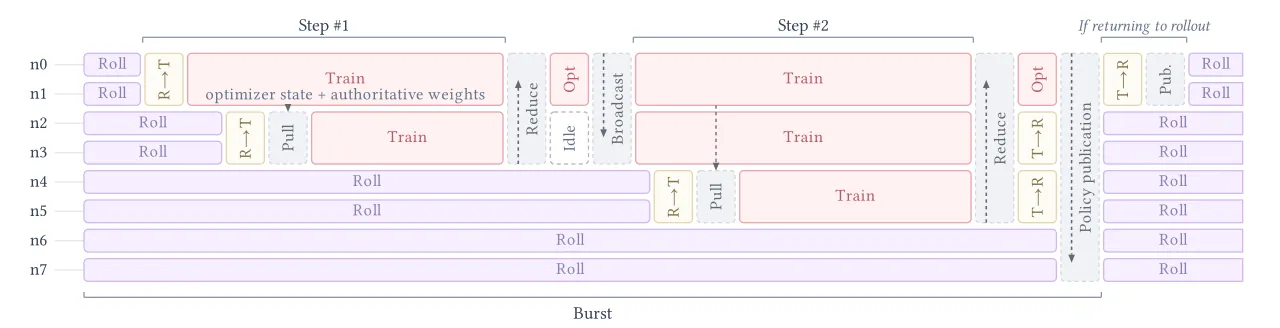
Figure 2: an illustrative timeline for a two-step burst (paper Figure 4). The core (n0-n1) completes two updates; satellites join an in-flight step after pulling current parameters; gradient reduction happens before every update, parameters are broadcast after each non-final update, and the rollout policy is published after the final one. The core's last role transition and local publication occur only if it returns to rollout.

Role transitions that keep the harness alive

During a role transition the harness, workspace and tool execution state stay in place while the proxy reroutes model calls. The source cell first stops accepting new requests; the scheduler reserves destination capacity for the affected executions and updates routing; unfinished requests on the source engine are then cancelled and transparently retried onto the destination engine by the proxy. Destination selection prefers the separate pool engine, then rollout cells in reverse index order, so that the destination expected to stay longer is chosen first and one execution is not rerouted repeatedly within a single burst.

KV-cache migration reduces the prefix recomputation caused by rerouting. Before a request is cancelled on the source engine the source pins the corresponding cache blocks; after cancellation completes and cache writes stop, the destination reads those blocks over RDMA; the source releases them only once the destination confirms it has taken over. When the transition completes the cell offloads rollout parameters and frees KV cache and scratch buffers to reclaim memory, then restores training parameters and buffers. Backend processes and communication groups stay alive across the whole role change, so transition overhead is only seconds: 8.52 s on average from rollout to training and 3.46 s from training to rollout, negligible against executions that last hours.

Streaming training with dynamic membership

To let a satellite join a batch already in flight, the core exposes a buffer holding the authoritative weights through the Mooncake Transfer Engine when it moves from rollout into training and again before each subsequent step. A satellite registers with the scheduler, pulls core weights over RDMA and starts training immediately without interrupting the core. Weights are frozen during gradient accumulation, so a joiner reads a self-consistent snapshot, and the controller closes the join window before the optimizer update. For $K$ ordered cells the system pre-builds $K-1$ communication groups, one for each prefix of $2,\ldots,K$, and collective communication selects the group matching the participating prefix. After the batch is processed the core aggregates and normalizes gradients from all training cells, clips them and performs a single optimizer update, broadcasting the new parameters to the current satellites after every non-final update.

Streaming training relies on two buffers. The trajectory buffer stores execution records and rewards per rollout group. The stream packing buffer pulls one ready group from the trajectory buffer when it runs short of trajectories, preferring the oldest policy version, materializes the selected trajectories into token rows, reorders them for efficient packing and emits training input in units of micro-steps. Cells claim micro-steps atomically from a shared queue whenever compute frees up, so they receive disjoint work; earlier or faster cells consume more micro-steps, which makes participating cells finish the same batch at roughly the same time. The packing buffer selects the $B$ groups of a batch incrementally and closes the stream only after all their micro-steps are enqueued. Each cell processes micro-steps with a continuous one-forward-one-backward pipeline; when data is momentarily missing every stage stops at a consistent scheduling point after finishing in-flight communication while keeping pipeline state; once the stream is closed and the queue drained the pipeline flushes remaining work, so each cell pays exactly one warmup and one drain per batch.

flowchart TD
  HB[Harness in sandbox
unmodified black-box agent] -->|model calls| PX[Black-box proxy
records TITO tokens and behavior log-probs]
  PX --> RT[Rollout engines
SGLang cells in rollout role]
  RT -->|responses| PX
  PX ==> TT[Trajectory trees
shared prefixes keep original contexts]
  EV[Evaluator
scores preserved workspace
valid partial progress after timeout] ==> BF[Trajectory buffer
records and rewards by rollout group]
  TT ==> BF
  BF ==> PK[Stream packing buffer
admits at most Jmax paths per execution
shared targets counted once]
  WL[Rollout waterlevel
dispatched minus finished] -->|falls below remaining capacity| SC[Elastic scheduler
serial transitions core first
supply check rho_min and tau]
  SC -->|train role| TR[Training cells
satellites pull core weights via RDMA
claim micro-steps atomically]
  PK ==>|micro-steps| TR
  TR ==>|gradients| CORE[Core cell
single optimizer update per batch]
  CORE -->|publish weights at burst end| RT

Figure 3: control and data flow of QwenGyre (corresponding to Figure 3 of the paper). Thin control edges are burst-boundary actions and the waterlevel feedback drives role transitions; the thick edges are the data flow, where the two buffers carry trajectory storage and stream packing.

Trajectory processor: from execution records to trajectory trees

Under TITO the proxy saves the exact input and output token ids of each model call, the behavior log-probabilities of the output tokens and metadata. To maintain those records across the message handling of different harnesses the proxy also caches raw tool-call payloads keyed by call id and restores them before matching subsequent request histories, while keeping the incoming ids for tool-response correlation; this prevents spurious history mismatches caused by tool-call reformatting. The harness keeps using its own message interface, training consumes the recorded tokens and metadata, and every output keeps the context it was conditioned on even after that context is compacted away.

Request records are organized into one trajectory tree per execution: a node stores incremental input, recorded output and metadata. After tool-call restoration the framework matches the serialized context of an incoming request against existing paths, reuses stored tokens and encodes only the new content, appending the new record as a node; divergent contexts create branches and unmatched requests attach to the root. The real case in Appendix C, execution f3ad38e5 with 636 proxy requests, 1,347 unique message nodes and 10 candidate trajectories, shows that after the main agent and the catalog sub-agent each compact their history the shared prefixes reach 168 and 193 message nodes; the 10 complete paths hold 53 to 293 nodes each, and expanding them independently would produce 1,716 node occurrences, 369 more repetitions than the shared representation.

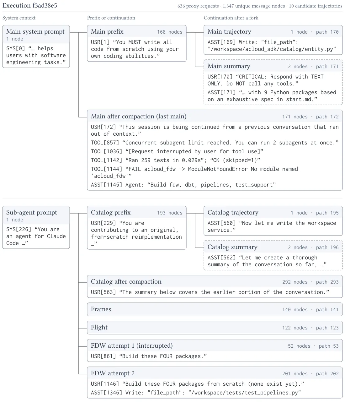
Figure 4: the prefix graph of execution f3ad38e5 with real message excerpts (paper Figure 12). Orthogonal edges encode prefix sharing and dashed boxes are summary leaves; the interruption at TOOL[1036] stays inside the main context that received it. The main agent and the sub-agent have separate roots because their system prompts differ, and causal parent-child relation is not the same thing as context prefix sharing.

Partial scoring: a timeout is neither zero nor invalid

When an execution closes, QwenGyre freezes the committed policy-generated request records, identifies the available artifact state and evaluates the preserved work under the task scoring rules, including after a timeout. An unfinished execution earns a valid score as long as its completed portion is evaluable, and for those evaluated outcomes the data plane derives no reward from elapsed time, trajectory length or termination status. The evaluator returns a score, a validity status and a reference to the evaluated state. An xLong execution may evaluate an intermediate artifact, revise it and abandon a branch, so every evaluation is bound to its execution, artifact version and available branch references, and later evaluations do not overwrite those associations. A critique that is later consumed as input by a policy request is excluded from the policy training objective precisely because of its evaluator provenance.

Failures are handled in three classes. An evaluator failure leaves the evaluation pending and may be retried on the same preserved state within the total time budget of the execution; when the budget runs out without a valid reward the recorded trajectory is excluded from training, since a pending evaluation is different from a valid zero score and the latter is still trainable. A rare total failure such as an image pull error leaves no evaluable work at all, and QwenGyre then inserts a dummy trajectory with zero reward as a failure placeholder so that the group counts stay complete. This distinction maps directly onto the requirement of group-relative advantages: a group has $N$ valid sample rewards only after every execution has closed and the designated outcome is valid.

Trajectory sampling: bounded paths by role priority

Trainable tokens are decided by provenance: only tokens generated by the policy during rollout are targets. TITO records whether each token was emitted by the SGLang engine or supplied externally; system prompts, user prompts, tool results and assistant content injected rather than sampled by the harness are all masked and kept only as conditioning context. Candidate trajectories correspond to leaves of the trajectory tree: a leaf plus the root-to-leaf prefix path defines one trajectory. Under xLong a single execution can produce many candidates and the count varies enormously across executions, so keeping them all would wreck training efficiency. QwenGyre therefore keeps at most $J_{\max}$ trajectories per execution, five by default, filling them in order of expected importance. For the Claude Code harness leaves are split into four classes by the role of their request sequence, with priority

$$\text{main} > \text{main-summary} > \text{sub-agent} > \text{sub-agent-summary}. \tag{4}$$

The order rests on two principles: turns of the main agent are the most direct credit-bearing object of the task-level reward while sub-agent trajectories contribute only indirectly through delegated subtasks, and within one agent the turns that advance the task rank ahead of the summary turns that merely manage context. Admission proceeds one draw at a time from the provenance mask: each step takes the highest-priority class that still has unmasked trainable tokens and draws one leaf with probability proportional to its unmasked token count; the targets of the drawn trajectory are frozen to exactly the tokens that are still unmasked at that moment, and the whole root-to-leaf path is then masked on the tree, so a shared prefix is never trained twice, already frozen targets are unaffected, and the reduced counts reweight the next draw. Admission repeats until no unmasked trainable token remains or $J_{\max}$ is reached, yielding $J_i\leq J_{\max}$ trajectories that each inherit the group-relative advantage of that execution.

flowchart LR
  T1[main task-driving leaves] -->|priority 1| AD[Admission loop
draw one leaf proportional to unmasked tokens]
  T2[main summary leaves] -->|priority 2| AD
  T3[sub-agent leaves] -->|priority 3| AD
  T4[sub-agent summary leaves] -->|priority 4| AD
  AD -->|fix targets then mask root-to-leaf path| MS[Shared prefix targets counted once]
  AD -->|stop at Jmax or no unmasked token| TRJ[Bounded trajectories
each inherits the execution advantage]

Figure 5: the admission rule on the tree. After each draw the whole root-to-leaf path is masked, so a shared prefix contributes exactly one training signal and the draw probabilities of the remaining leaves are reweighted accordingly.

Execution-level objective: one more trajectory does not add weight to an execution

For execution $i$ let $\mathcal{R}_i$ be the admitted trajectory set, and let the target set $\mathcal{T}_r$ of trajectory $r$ be frozen to the trainable tokens that were still unmasked when it was drawn; on-tree masking makes these sets disjoint. Write $\mathcal{T}_i=\bigcup_{r\in\mathcal{R}_i}\mathcal{T}_r$, $L_r=|\mathcal{T}_r|$ and $L_i=|\mathcal{T}_i|=\sum_{r}L_r$. The token importance ratio and the gradient-free execution-level sequence ratio are

$$\rho_u(\theta)=\frac{\pi_\theta(y_u\mid c_u)}{p_u^{\mathrm{roll}}},\qquad s_i(\theta)=\operatorname{sg}\!\left[\exp\!\left(\frac{1}{L_i}\sum_{u\in\mathcal{T}_i}\log\rho_u(\theta)\right)\right]. \tag{5}$$

Here $p_u^{\mathrm{roll}}$ is the recorded behavior probability, reused directly instead of being recomputed. $s_i(\theta)$ is used for monitoring only and, together with the sign of the group-relative advantage $\hat{A}_i$, decides one shared clipping mask $m_i(\theta)$: it is set to zero when $\hat{A}_i>0$ and $s_i(\theta)>1.005$, zero when $\hat{A}_i<0$ and $s_i(\theta)<0.995$, and one otherwise. The token-level importance weight is $\bar{\rho}_u(\theta)=\operatorname{sg}(\min\{\rho_u(\theta),5\})$ and may differ across tokens of the same execution; the token loss is capped at 100, giving $\ell_u(\theta)=\min\{100,\,-m_i(\theta)\bar{\rho}_u(\theta)\hat{A}_i\log\pi_\theta(y_u\mid c_u)\}$.

Normalization is what makes this design work. Weighting each trajectory by its target share $L_r/L_i$ and then averaging over its targets gives

$$\mathcal{L}_i(\theta)=\sum_{r\in\mathcal{R}_i}\frac{L_r}{L_i}\cdot\frac{1}{L_r}\sum_{u\in\mathcal{T}_r}\ell_u(\theta)=\frac{1}{L_i}\sum_{u\in\mathcal{T}_i}\ell_u(\theta), \tag{6}$$

so every admitted target receives the same coefficient $1/L_i$, and neither importance weighting nor clipping changes that denominator; an execution with $L_i=0$ contributes zero loss. At batch level the loss is averaged over the $N$ raw executions of all $B$ queries, $\mathcal{L}(\theta)=\frac{1}{BN}\sum_{q=1}^{B}\sum_{k=1}^{N}\mathcal{L}_{i(q,k)}(\theta)$. The aggregate normalized weight of one execution is thus independent of how many trajectories it contributes: for a fixed admitted target set $\mathcal{T}_i$, choosing a different selected path to carry a given shared target leaves the sequence ratio, the clipping decision and the loss of that execution unchanged. Sampling can change $\mathcal{T}_i$ itself, but the invariance concerns assignment and ordering for a fixed target set, and packing preserves these per-execution weights.

Experimental Results

Evaluation covers three agentic workloads: NL2RepoBench, which builds a software repository from a natural-language specification and, during training, scores generated code with a separate Qwen 3.7-Max evaluator against independently written tests; DeepSWE, software engineering inside existing repositories evaluated by repository tests; and TerminalBench, multi-turn terminal tasks evaluated by task-specific verifiers. All three run Claude Code 2.1.220 executing shell and file operations in a containerized environment. The models are Qwen 3.6 122B and the flagship Qwen 3.8 2.4T: 122B NL2RepoBench uses 32 nodes, eight 4-node cells by default and 144 concurrent executions per cell; DeepSWE and TerminalBench use 24 nodes, six cells and 192 concurrent executions per cell; 2.4T uses four 48-node cells with 384 concurrent executions in total. The RL algorithm is a GSPO variant with token-level importance correction: $N=16$ executions per group, $B=32$ groups per step on NL2RepoBench and $B=48$ elsewhere, a token importance ratio cap of 5, a sequence-level clipping interval of $[0.995,1.005]$, $J_{\max}=5$ and a constant Adam learning rate of $10^{-6}$. Baselines are Colocate and Async under the same GPU budget and the same target staleness, and both use boundary dispatch.

The execution profile of xLong explains why the scheduling design is necessary. On Qwen 3.6 122B, NL2RepoBench averages 1.93 hours per rollout execution and 2.96 hours per query, and 9.51% of queries exceed four hours; the harness timeout rate is 6.25% (results are still scored and used for training) and the overall timeout rate is 0.87% (budget exhausted, no valid reward, discarded). On Qwen 3.8 2.4T the timeout rates go up even though the timeout ceiling is relaxed: 61.1% of queries exceed four hours, and 38.2% of the longest rollout executions end in an overall timeout. A heavy tail coexisting with clustered terminations is exactly the shape waterlevel control is built for.

On end-to-end performance, 122B NL2RepoBench after 48 steps gives QwenGyre a 1.42-1.53× speedup over Async and 1.36-1.47× over Colocate at both staleness targets, with training score curves comparable to the baselines, so the speed does not come from trading away task performance. The role timelines show cells entering training at different moments while the rest keep rolling out, so training starts from a subset and then expands; the capacity a fixed Async partition leaves to rollout and the wait Colocate pays for switching its whole pool are both absorbed by that overlap. The gap is wider on 2.4T: 48 steps take QwenGyre 75.42 hours against 134.55 hours for Async and 91.47 hours for Colocate, that is 1.78× and 1.21×, while the evaluation pass rate rises from 52.48% to 58.54%. The smaller gain over Colocate has an explanation too: query durations cluster near the timeout ceiling, so QwenGyre has fewer chances to reclaim cells early, and Colocate already shares one resource pool with training. A fixed Async partition instead keeps capacity locked on the training side while training is idle, and QwenGyre hands that capacity back to rollout dynamically, which is where the larger gain comes from.

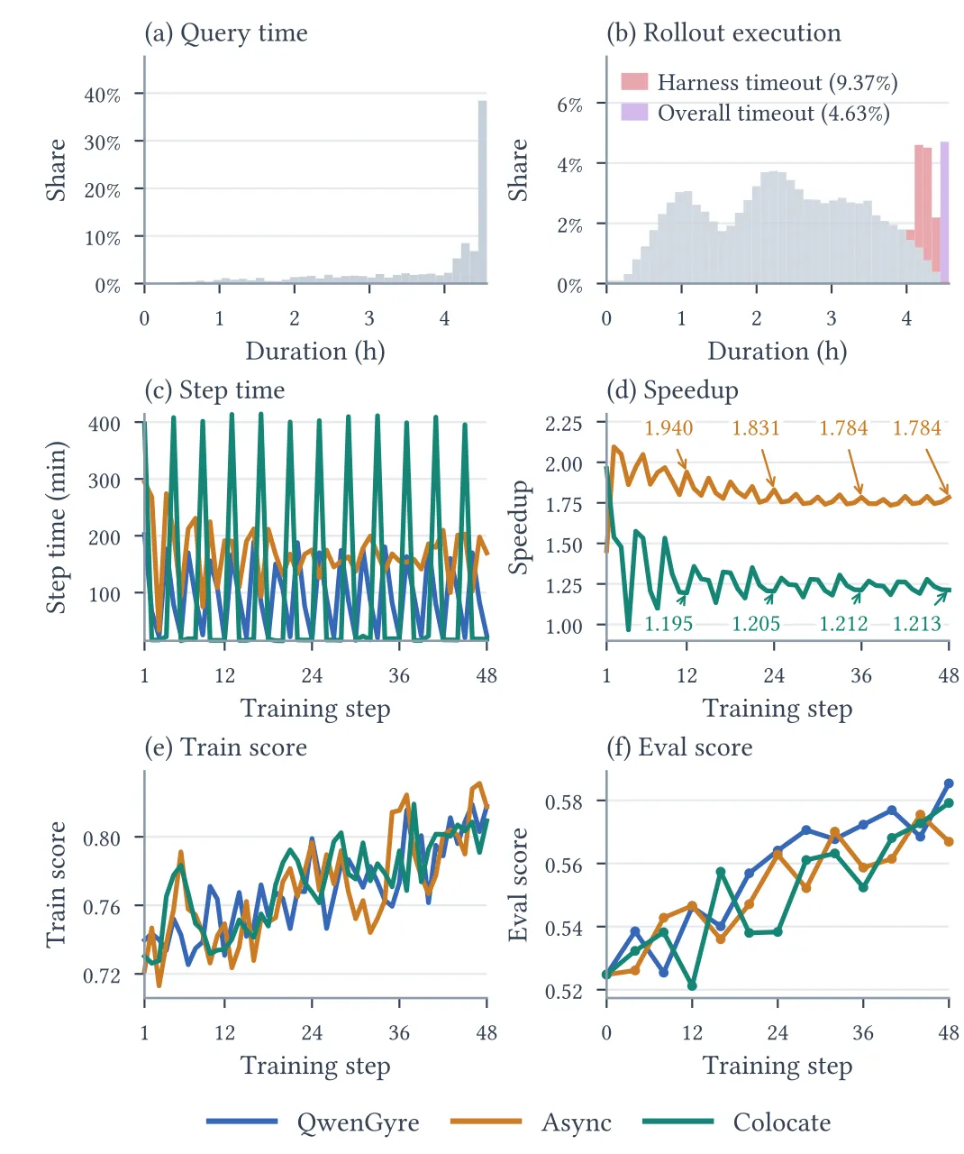
Figure 6: NL2RepoBench results on Qwen 3.8 2.4T (paper Figure 8). (a)(b) query and rollout execution duration distributions, last bin collects 4.45 h and above; (c)(d) step duration and cumulative speedup (Async 1.940 to 1.784, Colocate 1.195 to 1.213); (e)(f) training and evaluation scores, with the evaluation pass rate going from 52.48% to 58.54% within 48 steps.

Workload	Target 𝛚[d]	QwenGyre (φ,μ)	Speedup vs Async	Speedup vs Colocate
DeepSWE (24 steps)	1	(0.5, 2)	1.569	1.610
DeepSWE (24 steps)	1.5	(0.5, 3)	1.572	1.824
TerminalBench (24 steps)	1	(0.5, 2)	1.383	1.809
TerminalBench (24 steps)	1.5	(0.5, 3)	1.430	1.849
NL2RepoBench, 2.4T (48 steps)	—	—	1.78	1.21

Table 1: cumulative 24/48-step speedups across workloads (paper Table 2 and Figure 8). Async uses $(\varphi,\mu)=(\mathbb{E}[d],1)$ and Colocate uses $(0,2\mathbb{E}[d]+1)$, both balanced through $\mathbb{E}[d]=\varphi+\frac{\mu-1}{2}$.

The ablation splits QwenGyre into two evolutionary paths, adding streaming training to Async and adding separate rollout nodes to Colocate, before both converge on fine-grained elastic allocation. Moving nodes from training to rollout (A0 to A1) is actually 7.7% slower: executions complete in clusters, the smaller training pool digests them more slowly, and weight publication plus redispatch slow down with it. Lengthening the burst (A2) is 29.9% slower because the fixed rollout pool cannot supply it. Streaming training (A3) is 11.6% faster but only captures part of the benefit, since a fixed partition still cannot move GPUs as demand changes. On the Colocate side, adding separate nodes (C1) is only 2.9% faster than C0; adding streaming on top (C2) is 14.8% faster, yet the 28 colocated nodes still have to switch together and streaming can only start late in the burst; enlarging the separate pool (C3) leaves fewer training nodes and a longer training phase, ending up 7.6% slower than C2. E0 replaces the fixed split of C2 with eight independently switchable 4-node cells and is 1.19× faster than C2. E1 shortens the burst to one step, raising $\varphi$ from 0.5 to 1.5 to hold staleness constant, and is 10.9% slower than E0 but still 1.24× faster than A3, which also uses single-step plus streaming, and 1.08× faster than C2, so fine-grained allocation holds even without a multi-step burst. E2 reorganizes the same 32 nodes into four 8-node cells and is only 2.2% slower than E0, because in E0 rollout fully masks training with 20.85% slack left and coarse cells expose only a little training on the critical path.

ID	Evolution	Streaming	Transition granularity	(φ,μ)	Allocation	12-step total (h)	vs E0
A0	vanilla Async	off	—	(1.5,1)	16 T / 16 R	25.08	1.556
A1	A0 repartitioned	off	—	(1.5,1)	8 T / 24 R	27.01	1.676
A2	A0 + multi-step burst	off	—	(0.5,3)	16 T / 16 R	32.58	2.021
A3	A0 + streaming	on	—	(1.5,1)	16 T / 16 R	22.18	1.376
C0	vanilla Colocate	off	Global	(0,4)	32 C / 0 S	23.23	1.442
C1	C0 + separate rollout nodes	off	Coarse	(0.5,3)	28 C / 4 S	22.56	1.400
C2	C1 + streaming	on	Coarse	(0.5,3)	28 C / 4 S	19.23	1.193
C3	C2 reallocated	on	Coarse	(0.5,3)	16 C / 16 S	20.69	1.284
E0	C2 + fine-grained elastic cells	on	Fine	(0.5,3)	8 cells × 4	16.12	1.000
E1	E0 single-step burst	on	Fine	(1.5,1)	8 cells × 4	17.87	1.109
E2	E0 with four 8-node cells	on	Fine	(0.5,3)	4 cells × 8	16.47	1.022

Table 2: scheduling ablation over the first 12 NL2RepoBench training steps (paper Table 1, Qwen 3.6 122B, 𝛚[d]=1.5). T/R are training and rollout nodes, C/S are colocated and separate nodes; lower is better.

The trajectory budget ablation answers how many trajectories to train per execution. Training only the main trajectory is not enough: the first 42 steps show a lower training score and a larger gradient norm. Raising the budget to five matches the score of keeping every leaf trajectory while the gradient norm stays small as well. Over the same window the average forward-backward time per step is 41.4% of the uncapped baseline at cap=1 and 74.8% at cap=5, so cap=5 cuts 25.2% of the forward-backward time while holding the score. This is the other side of the normalization in Equation (6): extra trajectories do not add weight to an execution, but they recover the learning signal that compaction and delegation chopped up.

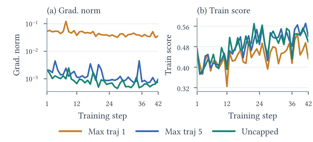
Figure 7: trajectory budget ablation over training steps 1-42 (paper Figure 9). (a) gradient norm on a log axis; (b) mean training score. Max traj 1 keeps only the main trajectory, Max traj 5 admits at most five, and Uncapped keeps every leaf.

Limitations

The first limitation stated by the authors concerns GPU budget and cell granularity: elastic scheduling needs several cells that can transition independently while still keeping enough rollout capacity to serve unfinished executions. Every cell must hold the model memory footprint and the training parallel requirements, so a small GPU budget cannot support this organization, and such deployments are unrealistic for xLong workloads anyway. Within the evaluated range a handful of cells is enough, since E2 is only 2.2% slower than E0 on the same 32 nodes, but efficiency at a substantially smaller total budget is not evaluated.

The second stated limitation is the conflict between streaming training and global shuffle. With $\mu>1$ streaming training hands ready groups to successive updates incrementally, so a global shuffle across all minibatches cannot be performed before the burst starts; supporting it would require waiting for the whole burst of data before the first update and would sacrifice the overlap with rollout. Training procedures that rely on globally random minibatch assignment are therefore constrained. A single-step burst ($\mu=1$) avoids the cross-minibatch split and keeps both elasticity and streaming, and E1 is 10.9% slower than E0 while still 1.24× faster than A3. The authors also concede that these ablations quantify execution time only, so the effect of sample ordering on learning quality is not isolated.

Two further observations of my own. First, the evaluation surface is narrow and tied to a single harness: all three workloads are software engineering or terminal tasks and every one of them runs Claude Code 2.1.220. The four-class role priority in Equation (4) is tailored to the main agent, sub-agent and summary structure of Claude Code, so a different harness with different compaction policy, delegation semantics or retry behavior would need the priority classes and provenance masks redefined, and the paper offers no cross-harness sensitivity analysis. Second, the comparison protocol: every speedup is measured under boundary dispatch at a matched mean target staleness, and Appendix A itself notes that the counting identity covers only the group-weighted mean staleness, leaving worst-case and token-weighted guarantees, resource saturation and concurrency-dependent latency outside the assumptions. The continuous-dispatch analysis, $\mathbb{E}_c[d]-\mathbb{E}_b[d]=1+R/B$, shows that both dispatch policies carry a cost, yet the framework commits to boundary dispatch, and the applicability boundary of that choice is left to future work.

Conclusion and Outlook

The contribution of QwenGyre can be grouped into three layers. At the scheduling layer, waterlevel and supply checks turn the GPU role into a resource that migrates with demand, while RDMA weight pulls and pre-built communication groups let a satellite join a batch already in flight. At the data layer, TITO and trajectory trees preserve the original conditioning context of every output, partial scoring turns the usable progress of a timed-out execution into a valid reward, and on-tree admission compresses a branching execution into bounded, deduplicated, weight-balanced training samples. At the validation layer, a flagship 2.4T model with 700K-token rollouts delivers a 52.5% to 58.5% pass-rate gain in 48 steps and end-to-end speedups of up to 1.85× and 1.78× across three workloads.

For teams doing agent post-training, the reusable conclusion of this paper is that a black-box harness is an interface design problem rather than an obstacle: as long as the proxy preserves token-level records and inference availability, scheduling and trajectory processing can both be done outside it, and decoupling the lifecycles of execution, role and sample is the precondition for fitting hour-long rollouts into online RL. The open questions are equally clear: elastic organization at a smaller budget, compatibility of global shuffle with streaming, priority and provenance rules across harnesses, and the effect of sample ordering on learning quality.

Decouple the harness execution, the GPU role and the training sample: execution state survives role transitions and recorded model calls materialize into training samples on demand. Only then does online RL for xLong horizons fit inside one cluster.