PAPER DEEP DIVE
Learning Montezuma's Revenge from a Single Demonstration
We propose a new method for learning from a single demonstration to solve hard exploration tasks like the Atari game Montezuma's Revenge. Instead of imitating human demonstrations, as proposed in other recent works, our approach is to maximize rewards directly. Our agent is trained using off-the-shelf reinforcement learning, but starts every episode by resetting to a state from a demonstration. By starting from such demonstration states, the agent requires much less exploration to learn a game compared to when it starts from the beginning of the game at every episode. We analyze reinforcement learning for tasks with sparse rewards in a simple toy environment, where we show that the run-time of standard RL methods scales exponentially in the number of states between rewards. Our method reduces this to quadratic scaling, opening up many tasks that were previously infeasible. We then apply our method to Montezuma's Revenge, for which we present a trained agent achieving a high-score of 74,500, better than any previously published result.
One-Sentence Summary
Turn a single human demonstration into a curriculum of increasingly hard starting states: each RL episode begins at a demonstrated state, the starting point moves backward as the agent succeeds, and the agent eventually plays the whole game without the demonstration, reaching 74,500 on Montezuma's Revenge.
Background and Motivation
Model-free reinforcement learning learns by trial and error. Policy-gradient and Q-learning methods start every episode from the environment's initial state and explore randomly; when a random sequence of actions happens to produce a reward, those actions become more likely. This works when rewards are dense. It breaks down when the first reward requires a long, precise sequence of actions, because random exploration almost never hits it.
The paper makes the difficulty concrete with a product of probabilities. Suppose reaching the first key requires five critical events: descending ladder 1, grabbing the rope, descending ladder 2, jumping over the skull, and climbing ladder 3. The probability of getting the key is the product of those five probabilities. Each factor is below one, so the product is dramatically smaller than any individual factor. The authors report that uniformly random actions in Montezuma's Revenge produce a reward only about once every half a million steps.
More generally, if the first reward requires a correct sequence of length $N$, a random agent needs on the order of $\exp(N)$ steps before it can expect to see that reward. This exponential scaling is the central obstacle in sparse-reward tasks and the reason hard-exploration Atari games remain a stress test for RL.
Prior work follows two broad routes. One improves exploration itself: pseudo-counts, intrinsic motivation, ensemble uncertainty, and prediction-error curiosity. The other imitates demonstrations, training the agent to reproduce demonstrated actions or states. Exploration bonuses have produced only limited gains on Montezuma's Revenge. Imitation can work, but it requires high-quality demonstrations, often several of them, and it risks inheriting a sub-optimal trajectory.
This paper takes a third route. It does not imitate the demonstration's actions; it borrows only the demonstration's states to reset the environment, decomposing a long-horizon exploration problem into a sequence of short-horizon problems. Rewards still come from the original environment and are optimized directly by RL. The agent therefore remains free to discover solutions the demonstrator never considered.
Preliminaries
Sparse rewards and the blind cliff walk. The analysis uses the blind cliff walk introduced by Schaul et al.: a one-dimensional cliff of $N$ states with two actions per state, one correct and one fatal. Only the final state yields a reward. The agent is assumed unable to generalize across states, so it must learn a tabular policy for each state independently. That makes the environment a clean sandbox for measuring exploration complexity.
Distributed PPO. Training uses PPO. Each rollout worker collects trajectories of fixed length $L$, and a centralized optimizer updates a shared recurrent policy with the clipped policy-gradient objective and a clipped value loss. The method does not invent a new optimizer; resetting from demonstration states is an algorithm-agnostic curriculum layer that can sit on top of PPO, A3C, or IMPALA.
Episodes, resets, and hidden state. For a recurrent policy, restoring the environment to a demonstrated frame is not enough: the policy's hidden state must reflect what just happened. The method therefore replays the $K$ demonstration transitions immediately preceding the chosen starting point, warming up the RNN state, and then hands control to the policy.
Method
1. Turn the demonstration into resettable states. Given a demonstration $\{(\tilde{s}_t,\tilde{a}_t,\tilde{r}_t,\tilde{s}_{t+1})\}_{t=0}^{T}$, each rollout worker starts an episode at a demonstrated state $\tilde{s}_{\tau^*}$. Early in training, every worker starts near the end $T$ of the demonstration, where success is only a few actions away and exploration is nearly trivial.
2. Move the starting point when the success rate is high enough. The optimizer measures the fraction of episodes whose return ties or beats the demonstration's return over the same segment:
$$\frac{\sum_{D} W_i}{\sum_{D} d_{i,t}} \ge \rho$$
Here $W_i$ counts successful episodes for worker $i$ and $d_{i,t}$ marks episode termination. The threshold is $\rho = 20\%$. Once the success rate clears it, the central starting point moves backward by a fixed step:
$$\tau \leftarrow \tau - \Delta$$
This dynamic adjustment is the paper's most important engineering decision. The authors state that they tried a predefined curriculum and found the dynamic version essential on a task as hard as Montezuma's Revenge.
3. Sample local starting points within a window. Workers do not all start at exactly $\tau$. Each samples its own $\tau^*$ uniformly from a small window $\{\tau-D,\ldots,\tau\}$ to preserve diversity. In the released code this is implemented by mapping each worker index to a different demonstration offset, spreading the parallel workers across the most recent segment of the demonstration.
4. Warm up the RNN by replaying K demonstration steps. After choosing $\tau^*$, the worker sets its time counter to $\tau^*-K$ and replays the demonstration transitions from that point up to $\tau^*$, feeding observations, actions, rewards, and done flags through the policy. These transitions are marked invalid and masked out of the training loss. The code uses an actions_to_overwrite queue and sets valid=False during replay; the loss then multiplies by the VALID mask. The hidden state is restored without teaching the agent to imitate the demonstrated actions.
5. Let the policy take over until the episode ends. After warm-up, the agent samples actions from the current policy $\pi(\theta)$ and interacts with the real environment. At the end of the episode, the segment return is compared with the demonstration return over the same segment:
$$\sum_{t \ge \tau^*} r_t \ge \sum_{t \ge \tau^*} \tilde{r}_t$$
If the inequality holds, the episode counts as a success. The implementation adds two practical termination rules that the paper does not emphasize: an episode ends after a small number of extra frames once the agent reaches the demonstration's final score, and it is killed if, after 50 actions, the agent's score lags the demonstration's return at the same point. Both rules concentrate compute on promising rollouts.
6. Finish with a demonstration-free agent. When the central starting point reaches $\tau=0$, the agent starts from the game's true initial state and finishes the run on its own. The demonstration no longer influences any decision. The authors interpret this as a form of dynamic programming: a long sequence is broken into $N$ short segments, each of which requires only a small improvement over what the agent can already do.
7. Complexity drops from exponential to quadratic. If each of the $N$ states takes $O(N)$ steps to learn, learning all of them costs $O(N^2)$; exploring from scratch costs $O(\exp(N))$. Figure 3 reports fits of $6.0 \cdot 2^{N}$ for the from-scratch curve and $47 \cdot N^{2}$ for the demonstration-initialized curve. These constants matter: at $N=18$ the gap spans more than two orders of magnitude.
8. The boundary with imitation learning. The method requires control over the environment and access to the demonstration's full states, but it does not require the demonstrated actions to be executable and does not force the policy to reproduce them. The restriction is real, but the payoff is that the objective stays the task return, so the agent can surpass the demonstration. In the reported run it scores 3,000 points above the human demonstration and exploits a game mechanism the authors did not know about.
flowchart TD
    A[Single human demonstration of length T] --> B[Set central start tau near the end]
    B --> C[Each worker samples local start in tau-D to tau]
    C --> D[Replay K demo steps to warm up RNN
and mask those transitions]
    D --> E[Policy takes over and samples actions]
    E --> F{Segment return >= demo return}
    F -->|yes| G[Increment success counter W]
    F -->|no| H[No success]
    G --> I{Success rate >= 20 percent}
    H --> I
    I -->|yes| J[Move tau back by Delta]
    I -->|no| K[Keep the starting point]
    J --> L{tau equals 0}
    K --> L
    L -->|no| C
    L -->|yes| M[Agent plays from the true initial state]
Experiments
Blind cliff walk: the complexity claim is measured, not assumed. The authors train tabular policies on cliff lengths from 1 to 18, require a 95% solve rate, and take the geometric mean over 20 random seeds. Figure 3 shows the from-scratch curve tracking the exponential fit and the demonstration-initialized curve tracking the quadratic fit. The two asymptotic regimes are visible on the same axis.
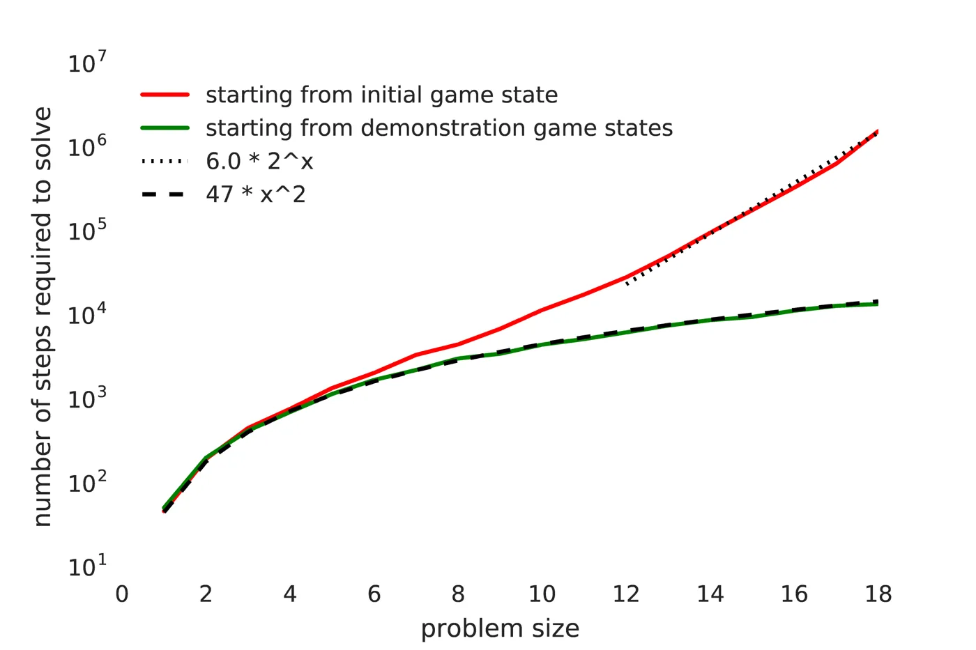
Figure 3: Steps required to solve the blind cliff walk. Red starts from the initial state, green starts from demonstration states; dashed lines fit $6.0 \cdot 2^x$ and $47 \cdot x^2$.
Montezuma's Revenge: one demonstration, 74,500 points. The demonstration was recorded with a tool that allows reversing game time and correcting mistakes; it scores 71,500 over roughly 15 minutes, still more than ten times below expert human scores achieved without such tools. The trained agent reaches 74,500 in about 12 minutes, beating the demonstration by 3,000 points. It exceeds the demonstration by collecting more diamonds and by exploiting a key-respawn mechanism at minute 4:25, a route the authors did not know about when recording.
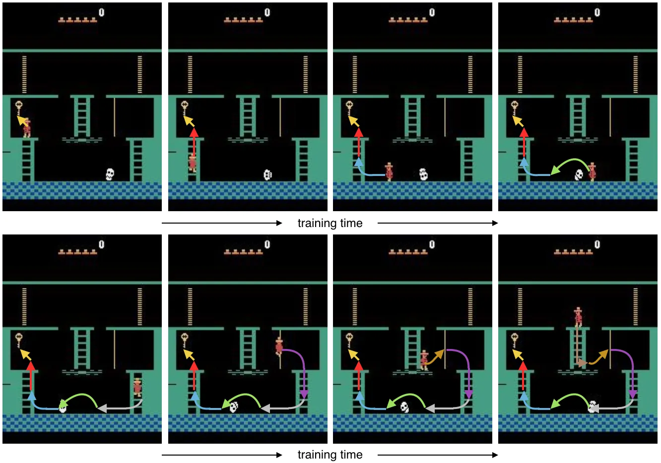
Figure 1: The starting state moves backward over training. The agent first learns a single jump to the key, then climbing, rope descent, the skull jump, and finally the full game from the initial state.
| Approach | Score |
|---|---|
| Count-based exploration (Ostrovski et al., 2017) | 3,705.5 |
| Unifying count-based exploration (Bellemare et al., 2016) | 6,600 |
| DQfD (Hester et al., 2017) | 4,739.6 |
| Ape-X DQfD (Pohlen et al., 2018) | 29,384 |
| Playing by watching YouTube (Aytar et al., 2018) | 41,098 |
| This work | 74,500 |
Training scale. The policy is much larger than a standard Atari network. It receives $105 \times 80$ grayscale frames, passes them through a $7 \times 5$ 2D convolution with stride $2 \times 2$ and 64 channels, then through four 3D convolutions with spatial kernels $5 \times 5$, $5 \times 5$, $5 \times 5$, and $5 \times 3$. Each 3D layer has a temporal kernel of 2 and a temporal stride that grows as $2^l$; the channel count doubles at every layer. Training uses PPO on 128 GPUs with 8 workers each, for 1,024 rollout workers and about 50 billion frames over two weeks.
| Item | Value |
|---|---|
| Observation | 105 × 80 grayscale |
| Architecture | 1 2D conv + 4 3D conv layers (temporal kernel 2) |
| Optimizer | PPO (GAE λ = 0.95, γ between 0.999 and 0.9999) |
| Parallelism | 128 GPUs × 8 workers = 1,024 rollout workers |
| Training frames | About 50 billion |
| Curriculum threshold ρ | 20% |
| Wall-clock training | About 2 weeks |
Robustness evaluation. To test whether the policy merely memorized the demonstration, the authors re-evaluate it under two perturbations: repeating the previous action with probability 0.25 (sticky actions), and taking a random action with probability 0.01. The averages drop to 10,000 and 8,400 respectively. The absolute numbers fall sharply, but the authors note that both remain above all previously published results. Inserting 0 to 30 random no-ops at the start of an episode does not significantly hurt results, and most rollouts still reach the demonstration's final score.
| Evaluation condition | Average score | Notes |
|---|---|---|
| Clean evaluation | 74,500 | Low-entropy sampling, about 12 minutes |
| Sticky actions (p = 0.25) | 10,000 | Repeat previous action with 25% probability |
| ε-greedy (ε = 0.01) | 8,400 | Random action with 1% probability |
| 0–30 random no-ops | No significant drop | Most rollouts still reach demo score |
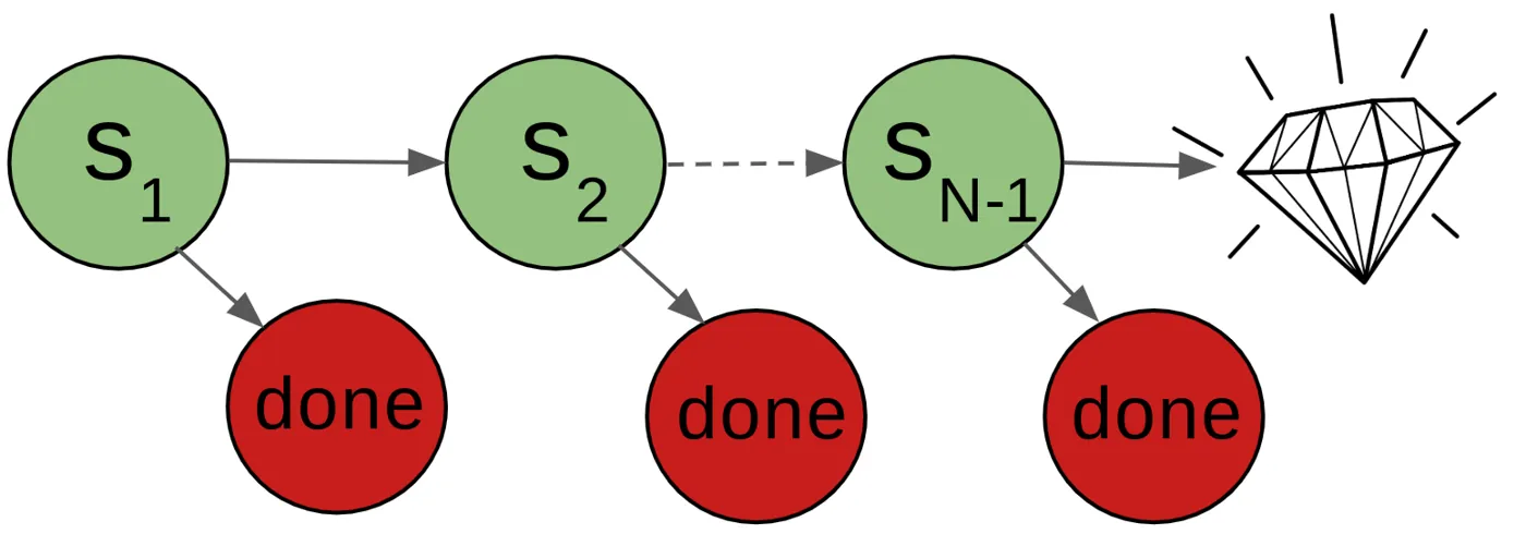
Figure 2: The blind cliff walk. Only one action sequence reaches the reward; every other action falls off the cliff, and each state is learned independently.
Limitations
1. It requires arbitrary environment resets. The method assumes the environment can be restored to any demonstrated state. That is easy in an Atari emulator and often expensive or impossible on a real robot. The authors acknowledge that imitation-learning approaches do not need this level of control; it is the method's hardest structural limitation.
2. States cannot be reproduced exactly. The authors note that an agent starting from an earlier state usually cannot reach the exact later state from the demonstration. Training uses a different frameskip from recording, and stochastic action sampling makes exact reproduction of an action sequence extremely unlikely. The policy must generalize across similar but non-identical states.
3. Cross-game generalization fails. The same pipeline works on Montezuma's Revenge but is much worse on Gravitar and Pitfall. Larger, deeper networks gave only partial improvement. The authors speculate that these games demand a harder vision problem but offer no systematic fix.
4. It is highly sensitive to hyperparameters. The paper states that PPO's entropy bonus had to be tuned carefully together with the learning rate and reward scaling to complete the curriculum. On Gravitar and Pitfall, the authors could not find a configuration that worked at all.
5. A single run, so variance is unknown. One training run costs 128 GPUs for two weeks, so the authors could not run independent seeds and report a single result. They explicitly list a systematic reliability study as future work, and this cost is easy to underestimate when attempting reproduction.
6. Scope relative to robotics. This is an Atari hard-exploration paper, not a robotics paper. Its value to embodied AI is methodological: the reset-based dynamic curriculum later became a common tool for manipulation and locomotion training in simulation, where arbitrary state resets are cheap.
Conclusion and Outlook
The contribution is not a larger network or a stronger exploration bonus. It is a reframing of what a demonstration is for: not a target to copy, but a set of launch points. By moving the episode start from the end of the demonstration back to its beginning, the method converts an exponential exploration problem into a sequence of short problems and lets a success-rate threshold drive the curriculum.
For embodied AI today, the idea is arguably more useful than it was in 2018. Simulators support arbitrary state resets, so manipulation and locomotion tasks can slice expert trajectories into segment starts and train with a reverse curriculum. On real robots, the hard part becomes cheap resetting, which is exactly the problem that reset-free learning and demonstration-initialized curricula attempt to solve.
Three natural extensions follow. First, replace the fixed success threshold with a curriculum that adapts to the policy's current competence. Second, combine state resets with a small amount of online correction so the method does not require full state access. Third, study approximate resets on real robots, such as a human placing objects back into a target configuration, and measure whether the quadratic scaling benefit survives.
Golden Quote
A demonstration is not an answer to memorize. It is a set of launch points; the path that matters is still the one the agent discovers for itself.