PAPER DEEP DIVE
RAVEN: A Unified Active SLAM System for Rapid Autonomous Visual Exploration with Aerial Robots under Localization Uncertainty
Active simultaneous localization and mapping (SLAM) addresses the problem of planning robot motion to build complete and accurate maps of unknown environments through efficient exploration while maintaining high localization accuracy. This raises a dilemma between exploring unknown spaces to expand coverage and exploiting visited regions to perform active loop closures. Despite numerous prior works on ground robots, aerial robots with high agility and constrained sensor suites face more significant localization drift and thereby demand dedicated active SLAM planning. Moreover, a unified strategy that adapts performance based on task-specific priorities remains an open question. In this article, we introduce RAVEN, a unified active SLAM framework for Rapid Autonomous Visual ExploratioN using quadrotors, which systematically accounts for localization uncertainty. The framework starts with identifying frontiers and active loop closure candidates, from which global tour candidates are generated. These candidates are evaluated using a utility vector that separately quantifies exploration efficiency and localization accuracy, and the final tour is selected according to a prioritization parameter ranging from [0,1]. Finally, a perception-aware navigation planner generates smooth execution trajectories that minimize visual state estimation error based on the online Fisher information field that provides visual localization information in real-time. Benchmark evaluations demonstrate that RAVEN outperforms state-of-the-art active SLAM methods, highlighting its advantages in producing a spectrum of performance across prioritizations. Fully onboard field experiments with a customized stereo-inertial quadrotor further validate its practical applicability in challenging environments. The source code will be released to benefit the community.
Paper metadata: Xinyi Chen, Yichen Zhang, Chenxing Jiang, and Shaojie Shen, Department of Electronic and Computer Engineering, The Hong Kong University of Science and Technology. arXiv 2610.37111, submitted 27 October 2026.
Paper: https://arxiv.org/abs/2610.37111. The authors state that source code will be released, but no official RAVEN repository was found when this analysis was prepared. Third-party SLAM components should not be mistaken for an official implementation.
Executive summary
RAVEN treats autonomous exploration and active loop closure as parts of one planning problem rather than two behaviors switched by hand-tuned thresholds. It builds a small set of high-quality global tours from frontiers and loop-closure candidates, evaluates each tour separately for completion time and expected pose-graph information, and selects a Pareto-optimal route according to a user-specified priority. During execution, an online Fisher information field steers both the flight path and camera yaw toward viewpoints that are more informative for visual localization.
Why aerial active SLAM needs a different planning stack
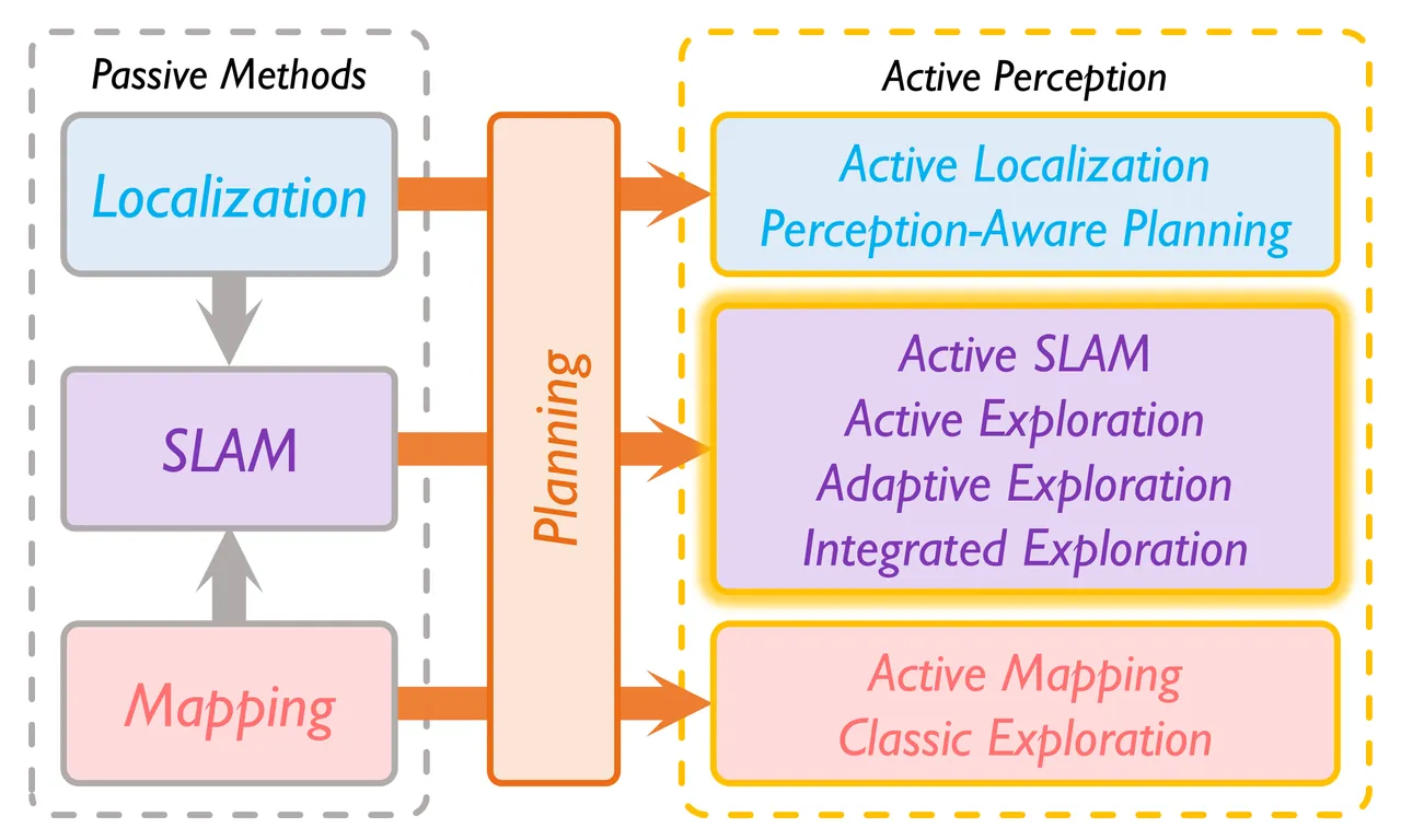
Classical exploration asks a robot to cover unknown space as quickly as possible under the simplifying assumption that localization is already reliable. Active SLAM removes that assumption. The robot must decide not only where the map boundary is, but also when a detour to a previously visited place will reduce state uncertainty enough to justify its cost. For a quadrotor, this choice is unusually consequential: fast motion produces rapid viewpoint changes, the camera has a limited field of view, and onboard visual-inertial odometry can accumulate substantial drift in long corridors or texture-poor rooms.
A common heuristic activates loop closure when estimated uncertainty crosses a threshold. This requires environment-specific tuning and reduces a continuous trade-off to a discrete mode switch. Another family of methods combines exploration gain and localization gain in a single utility function. Such a score can work well in a fixed setting, but its weighting has little physical meaning across maps whose spatial scale, feature density, or mission priorities differ. RAVEN instead preserves the two objectives and makes the trade-off explicit through a normalized priority parameter.
The aerial setting also exposes a second weakness in many active SLAM pipelines. Selecting an informative historical pose does not guarantee that the aircraft will remain well localized while flying there. If the local trajectory hugs a blank wall or points the camera away from tracked structure, localization can deteriorate before the loop closure is attempted. The planner must therefore control both the discrete decision to revisit and the continuous visual observability of the motion used to execute that decision.
RAVEN is organized around this distinction. Frontiers and active loop-closure candidates define possible intentions. Global tours assign them to a long-horizon coverage plan. A probabilistic virtual pose graph evaluates their localization value. Finally, a perception-aware local planner produces a feasible trajectory intended to preserve visual state estimation quality. Replanning occurs when frontier visibility changes, a trajectory finishes, or a periodic timer expires.
System representation and the compact pose graph
The online SLAM layer combines visual-inertial odometry, loop detection, and volumetric mapping. RAVEN does not require a particular underlying graph or particle-filter implementation. It compresses the high-frequency odometry history into a condensed pose graph whose nodes are six-degree-of-freedom camera poses sampled at a fixed geodesic interval. Consecutive edges carry relative-transformation covariance accumulated from the intermediate visual keyframes, and a detected loop adds a constraint between the corresponding historical and current regions.
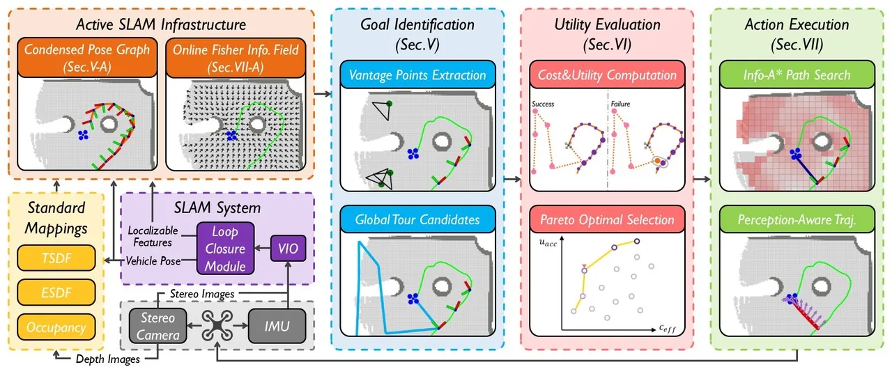
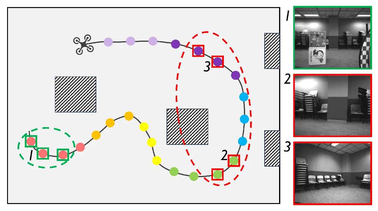
The condensed graph has two jobs. It reduces the cost of reasoning over a long trajectory, and it provides marginal covariances for deciding whether a proposed revisit is likely to succeed. This second role is essential: two poses can look similar in a NetVLAD embedding while the estimated uncertainty between their visits is still too large for a geometric loop constraint to be accepted.
RAVEN's contribution is therefore not a new visual SLAM back end. It is a planning architecture that consumes the compact graph and map maintained by a visual SLAM system. At each replanning cycle, the current graph is the starting point for evaluating hypothetical future visits. The architecture is designed to preserve uncertainty information from the SLAM estimate while keeping the planner's candidate set finite.
Goal identification: frontiers, loop candidates, and global tours
Frontiers are extracted as boundaries between known free space and unknown space. Active loop-closure candidates come from the trajectory history. RAVEN first clusters condensed-graph nodes that observe similar regions through feature covisibility and chooses the node seeing the most covisible features as each cluster representative. It then queries visually similar nodes with NetVLAD descriptors and Faiss. A representative is retained as a candidate only when the retrieved frames are concentrated in space; dispersed matches are more likely to come from repetitive texture or an unreliable visual alias.
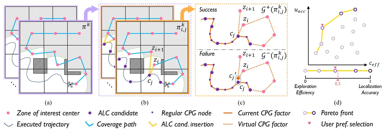
A one-step choice among the nearest frontier and the most informative loop closure would remain shortsighted. A detour can fragment a future coverage route even if its immediate information gain is high. RAVEN therefore decomposes the remaining map into connected zones and treats zones containing frontiers or unknown space as zones of interest. It solves a coverage route through their centers as an asymmetric traveling-salesman problem and keeps the best few base tours.
The active loop candidate is then inserted only into promising edges of those base tours. The paper deliberately inserts only the next upcoming loop closure rather than searching all combinations of several future revisits. This produces a manageable candidate set and enforces a useful property: removing the loop-closure detour should still leave a strong solution to the classical exploration problem. The global tour is consequently an exploration plan first, augmented with a bounded localization action.
Evaluating a tour without hiding the trade-off
For a tour that inserts loop candidate $c_j$ between zones $z_i$ and $z_{i+1}$, the expected exploration time is the base-tour duration plus the detour cost:
$$c_{\mathrm{eff}}(\pi_{i,j}^{k})=c_{\mathrm{eff}}(\pi^{k})+t(z_i,c_j)+t(c_j,z_{i+1})-t(z_i,z_{i+1})$$
Here $\pi^{k}$ is the base tour and $t(\cdot,\cdot)$ is distance divided by maximum speed. This cost is directly interpretable in seconds and accounts for the fact that a loop closure replaces part of the original inter-zone connection rather than adding an isolated round trip.
The localization value is calculated from a virtual extension of the current condensed pose graph. If the loop succeeds, new graph edges connect the historical candidate to virtual nodes generated by the upcoming route. If it fails, the route continues as a new trajectory and the aircraft receives no historical constraint. The graph is truncated after the following zone because only one loop closure is committed by the current global tour. Future graph structure will be recomputed with fresh observations.
RAVEN then estimates whether the revisit can actually produce a valid constraint. Let $\tilde{\Sigma}$ be the covariance of the difference between the marginal pose estimates at the two visits. For the differential-flat state components $w\in\{x,y,z,\psi\}$, the difference is modeled as zero-mean Gaussian. The success probability is:
$$p_{\mathrm{succ}}=\prod_{w\in\{x,y,z,\psi\}}P\left(|\tilde{w}|\lt\delta_w\mid \tilde{w}\sim\mathcal{N}(0,\tilde{\sigma}_w)\right)$$
The threshold $\delta_w$ defines an acceptable position or yaw discrepancy, and $\tilde{\sigma}_w$ is the corresponding variance. The expected localization utility is therefore a probability-weighted mixture of the successful and failed virtual graphs:
$$u_{\mathrm{acc}}(\pi_{i,j}^{k})=p_{\mathrm{succ}}h(\mathcal{G}^{+})+(1-p_{\mathrm{succ}})h(\mathcal{G}^{-})$$
where $h$ is an approximate D-optimal graph information score. The failed branch matters. A highly informative loop that is unlikely to be recognized contributes little expected accuracy and should not dominate planning simply because its best-case graph looks attractive.
Pareto selection makes λ operationally meaningful
Exploration time should be minimized, while pose-graph information should be maximized. These objectives have incompatible units. RAVEN avoids an arbitrary scalar sum by defining Pareto dominance. A candidate $\mathbf{x}$ dominates $\mathbf{y}$ when it is no worse on every objective and strictly better on at least one:
$$\mathbf{f}(\mathbf{x})\succ\mathbf{f}(\mathbf{y})\iff f_i(\mathbf{x})\geq f_i(\mathbf{y})\ \forall i,\quad \exists j:f_j(\mathbf{x})\gt f_j(\mathbf{y})$$
The non-dominated tours form a Pareto front. RAVEN interpolates along that front according to a priority parameter and selects the nearest candidate:
$$\mathcal{P}_{t:t+k}=\operatorname{Argmax}^{\succ}_{\mathbf{a}_{t:t+k}\in\mathcal{A}^{k}}\sum_{\tau=t}^{t+k}\mathbf{u}(b(\mathbf{s}_{\tau}),\mathbf{a}_{\tau}),\qquad \mathbf{a}^{\star}=S(\mathcal{P}_{t:t+k},\lambda)$$
A value near zero favors the shortest exploration tour. A value near one accepts extra travel and more loop closures to improve localization. Intermediate values interpolate the desired behavior. The parameter is not presented as a universal optimum that the algorithm discovers automatically; it expresses a mission-level preference that operators can reason about.
| Priority | Dominant behavior | Expected consequence | Representative use |
|---|---|---|---|
| λ = 0.0 | Cover unknown space quickly | Fewer active loops, shorter flight | Time-critical search with acceptable drift |
| λ = 0.5 | Balance coverage and revisits | Moderate detours and graph information | General autonomous exploration |
| λ = 1.0 | Protect localization accuracy | Frequent loops and longer trajectories | Inspection or reconstruction where geometry matters |
After selection, a loop-closure action directly targets the historical pose. An exploration action instead samples viewpoints around the target zone and chooses one that provides good frontier visibility and sufficient information from the online field. The long-horizon decision and the local observation choice are coupled rather than planned independently.
The online Fisher information field
Fisher information measures how strongly measurements constrain unknown parameters. For observation vector $\mathbf{x}$ and parameters $\boldsymbol{\theta}$, the observed information is:
$$\mathcal{I}_{\boldsymbol{\theta}}(\mathbf{x})=\frac{1}{\sigma^2}\mathbf{J}_{\boldsymbol{\theta}}^{\mathsf{T}}\mathbf{J}_{\boldsymbol{\theta}},\qquad \mathbf{J}_{\boldsymbol{\theta}}=\frac{\partial\mathbf{x}}{\partial\boldsymbol{\theta}}$$
The inverse Fisher information gives the Cramér-Rao lower bound for an unbiased estimator, so more information corresponds to a better attainable covariance. Recomputing the full matrix from every mapped feature at every candidate pose would be too expensive for online exploration. RAVEN's online field stores a rotation-independent positional factor in each free voxel and applies a rotation-dependent visibility query when a camera pose is evaluated.
The paper chooses a right-perturbation Jacobian. This avoids a scale artifact of the left-perturbation formulation: features with identical camera-frame coordinates can receive very different information scores when they are moved far from the world origin. With right perturbation, the trace has a compact closed form:
$$\operatorname{Tr}(\mathcal{I}^{R}(\mathbf{p}_i))=\frac{2}{n_i^2}+2,\qquad n_i=\lVert\mathbf{p}_i^{c}\rVert_2$$
The resulting score depends on the feature depth in the camera frame and remains invariant to camera rotation after taking the trace. This property is important because the field must compare voxels and trajectories across rooms that do not share a meaningful origin.
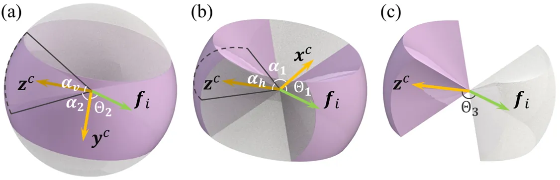
Visibility is represented by a smooth frustum model with separate horizontal and vertical field-of-view parameters. Gaussian-process regression over quaternion rotations decomposes the visibility term into a positional component and a rotational component. The positional component is accumulated in the voxel, while the rotational query multiplies it at planning time. In compact form, the total information is approximated as:
$$\mathcal{I}_{\mathbf{T}_{\mathrm{wc}}}\approx g\left(\sum_{i\in F}h(\mathbf{t}_{\mathrm{wc}},\mathbf{p}_i^{w}),\mathbf{R}_{\mathrm{wc}}\right)$$
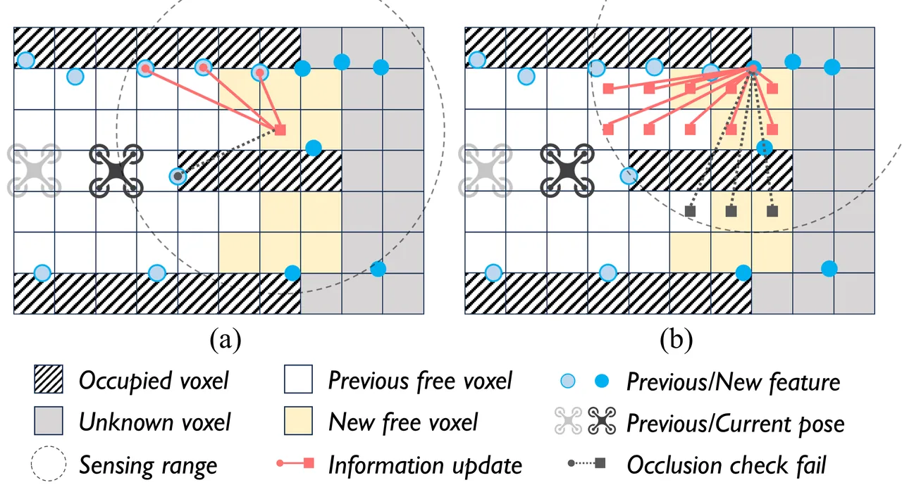
Updating the field requires identifying features that are useful for localization rather than every tracked pixel. A localizable feature must be observed and matched consistently over consecutive frames, giving it low positional uncertainty. When a new free voxel appears, existing localizable features within sensing range update that voxel. When a new localizable feature appears, it updates all nearby free voxels after occlusion checks. The two directions are necessary because exploration continuously creates both new observations and new query locations.
Translating information into a flyable trajectory
The planner defines an information potential that is flat above a sufficient-information threshold, rises quadratically near the threshold, and becomes strongly penalizing when information is extremely low:
$$f_{\mathrm{info}}(\mathbf{T})=\begin{cases}0,&\epsilon_{\mathrm{info}}\lt x\\k_1(x-\epsilon_{\mathrm{info}})^2,&0\leq x\leq\epsilon_{\mathrm{info}}\\k_2x+b_{\mathrm{pot}},&x\lt0\end{cases},\qquad x=\operatorname{Tr}(\mathcal{I}_{\mathbf{T}})$$
Because a quadrotor is differentially flat, position and yaw are optimized separately. The position planner first runs an information-aware A* search. Its cost combines geometric distance with the potential evaluated at the most informative sampled yaw at each node. This changes the initial homotopy: a path through feature-rich structure can be preferred over a marginally shorter path through a featureless corridor. The resulting path initializes a minimum-time B-spline subject to collision, smoothness, and dynamic constraints.
Yaw planning then samples candidate headings at knots along the position trajectory. A graph connects adjacent heading sets, with edge cost combining information potential and angular change:
$$f_{\mathrm{yaw}}=f_{\mathrm{info}}(\mathbf{P}_{i+1},\psi_{i+1,j_2})+w_{\mathrm{ys}}\operatorname{diff}(\psi_{i,j_1},\psi_{i+1,j_2})$$
Dijkstra's algorithm supplies a discrete yaw primitive path. That path initializes a smooth B-spline yaw optimization:
$$\min_{\Xi}\int_{t_0}^{t_m}\dddot{\psi}(t)^2\,dt+\lambda_p\sum_{i=1}^{m-1}f_{\mathrm{info}}(\mathbf{P}_i,\psi(t_i))$$
The first term penalizes yaw jerk; the second rewards headings with useful visual information. The two-stage procedure reduces sensitivity to local minima because the continuous optimizer starts from a globally searched heading sequence. Perception is therefore not just a reward attached to the final target. It shapes the route flown and the direction the camera maintains along that route.
flowchart TD
  A["VIO plus loop closure"] --> B["Condensed pose graph and volumetric map"]
  B --> C["Frontier goals"]
  B --> D["Active loop candidates"]
  C --> E["Candidate coverage tours"]
  D --> F["Insert next active loop"]
  E --> F
  F --> G["Success virtual graph"]
  F --> H["Failure virtual graph"]
  G --> I["Expected exploration time and graph information"]
  H --> I
  I --> J["Pareto front"]
  J --> K["Tour selected by lambda"]
  K --> L["Online Fisher information field"]
  L --> M["Info-A star position path"]
  L --> N["Yaw primitive graph"]
  M --> O["Constrained B-spline trajectories"]
  N --> O
  O --> P["Flight and new observations"]
  P --> A
Simulation benchmark
The authors extend the open EPEE exploration benchmark into EPEE+, adding multi-camera color rendering, configurable IMU noise, and visual SLAM. This matters because active SLAM cannot be evaluated fairly with perfect localization or synthetic drift unrelated to visual observations. Four scenes are used: corridor, warehouse, office, and apartment. Each planner is run ten times per scene with VINS and the same loop-detection components.
| Scene | Planner | Mean time (s) | Mean ATE (m) | Mean distance (m) | Looped image pairs |
|---|---|---|---|---|---|
| Corridor | FALCON | 74.8 | 0.43 | 78.1 | 16.8 |
| Corridor | RAVEN, λ=0.5 | 109.8 | 0.13 | 99.4 | 87.2 |
| Warehouse | FALCON | 87.7 | 0.55 | 90.7 | 11.3 |
| Warehouse | RAVEN, λ=0.5 | 107.4 | 0.17 | 96.1 | 65.2 |
| Office | FALCON | 64.6 | 0.49 | 61.0 | 12.6 |
| Office | RAVEN, λ=0.5 | 95.2 | 0.14 | 75.1 | 105.3 |
| Apartment | FALCON | 106.5 | 0.21 | 82.3 | 328.7 |
| Apartment | RAVEN, λ=0.5 | 136.9 | 0.13 | 104.7 | 675.8 |
FALCON remains the fastest planner because it optimizes exploration under a perfect-localization assumption. RAVEN at λ=0 stays close to that speed while reducing drift through perception-aware execution. As λ rises, RAVEN spends more time and distance on loop closure. At λ=1, its mean ATE reaches 0.08 m in the corridor, warehouse, and office and 0.08 m in the apartment. The important result is not only a better average at one operating point; the method produces a controlled spectrum between speed and accuracy.
SRE, REAL, and ExplORB are generally slower and less accurate in these trials. The authors attribute this to oscillatory revisiting and to local execution that does not account for feature distribution. RAVEN and FALCON define the time-accuracy Pareto front in all four scenes, but they occupy different portions of it: FALCON supplies the fastest endpoint, while RAVEN supplies progressively more accurate alternatives.
Two ablations isolate the mechanism. Replacing the perception-aware local planner with a perception-agnostic variant increases average ATE by 12.74% to 64.19% across tested priorities, while reducing exploration time by only 1.48% to 4.26%. In the loop-probability ablation, assuming every loop succeeds produces a final ATE of 0.45 m, thresholding candidates at 0.7 produces 0.46 m, and probability-weighted evaluation produces 0.09 m with 150.6 looped image pairs. The probability model is therefore doing more than re-ranking visually similar places; it prevents optimistic but infeasible loops from controlling the route.
Fully onboard field experiments
The field platform is a customized 1.3 kg quadrotor with an Intel i7-1260P mini PC, NxtPx4 autopilot, forward-facing RealSense D435i, and 6S battery. Planning, localization, mapping, and control run entirely onboard. Tests take place in a cluttered flight arena with motion-capture ground truth, a campus hallway containing cylindrical pillars and blank walls, and a larger underground parking lot.
| Scene | λ | Time (s) | Distance (m) | ATE or NND (m) | Looped pairs | Graph information |
|---|---|---|---|---|---|---|
| Flight arena | 0.0 | 44.8 | 33.6 | 0.18 | 4.40 | 16.1 |
| Flight arena | 0.5 | 48.7 | 38.2 | 0.14 | 17.8 | 20.1 |
| Flight arena | 1.0 | 51.5 | 39.3 | 0.10 | 36.6 | 25.2 |
| Campus hallway | 0.0 | 61.2 | 57.6 | 0.28 | 23.7 | 18.1 |
| Campus hallway | 0.5 | 80.8 | 67.7 | 0.21 | 67.3 | 29.3 |
| Campus hallway | 1.0 | 107.0 | 86.7 | 0.14 | 168.0 | 46.6 |
| Parking lot | 0.0 | 175.0 | 153.0 | 0.48 | 19.0 | 11.0 |
| Parking lot | 0.5 | 182.0 | 149.0 | 0.22 | 36.0 | 13.6 |
| Parking lot | 1.0 | 242.0 | 196.0 | 0.18 | 167.0 | 24.5 |
The flight arena has motion-capture trajectory truth. The hallway and parking lot do not, so the paper compares reconstructed maps against a handheld laser point cloud and reports nearest-neighbor distance. In the hallway and parking lot, increasing λ from 0 to 1 reduces mean NND by 50% and 62.5%, respectively. Visual inspection is consistent with the metric: cylindrical pillars and rectangular walls are distorted at low priority and substantially better preserved at high priority.
The large forest simulation covers an 80 by 20 by 2 meter scene with dense vegetation and uneven ground. RAVEN at λ=0.5 explores for 1081.6 seconds over a 759.6 meter trajectory and finishes with 0.664 meter ATE. CPG and OFIF updates run periodically in separate threads, leaving an average replanning time of 0.057 seconds with no clear growth over the run. Peak memory is 2.8 GB. These numbers support practical scalability for the tested scene, not a universal guarantee.
Limitations and open questions
The first boundary is explicit in the paper: RAVEN is designed for visually tractable environments under normal indoor illumination. It is not intended for spaces with almost no usable visual features, where visual SLAM becomes fundamentally infeasible. The information field can avoid texture-poor regions, but it cannot manufacture observations that do not exist. LiDAR, radar, or other modalities would be needed in those conditions.
The second boundary is approximation. The field scalarizes Fisher information by its trace, separates visibility through a smooth frustum and quaternion Gaussian process, and limits incremental updates to a local sensing neighborhood. The global candidate generator inserts only the next loop closure into each base tour. These choices make online planning tractable, but they do not represent the full combinatorial problem of planning many loops over a long horizon. Dynamic scenes, severe occlusion, and very large maps deserve further stress testing.
Third, the evaluation emphasizes exploration time, trajectory or map error, and graph information. Energy, control margin, emergency behavior, and dynamic-obstacle safety are not evaluated as first-class objectives. In field tests without trajectory ground truth, nearest-neighbor map distance is a reasonable geometric proxy but is not equivalent to trajectory ATE. Results should therefore be compared within their stated metrics and scene sizes.
Finally, λ is intentionally a mission preference rather than an automatically optimal value. Search-and-rescue may value speed, while structural inspection may prioritize map fidelity. The method makes that choice visible and reproducible, but deployment still requires selecting λ from mission risk, validating loop thresholds, and ensuring that the perception-aware trajectory remains safe under the actual vehicle dynamics.
Assessment
RAVEN's strongest idea is the causal chain it preserves. Localization uncertainty affects which historical poses are credible loop candidates, which global tours are selected, and how the aircraft flies toward the next target. The system does not assume that a good discrete goal automatically yields a good continuous trajectory. Probability weighting, Pareto selection, and the online information field each address a different failure point in that chain.
The work is also disciplined about what it approximates. It does not search an unbounded space of future loops, and it does not claim perception-aware control can rescue an entirely textureless environment. Those limits make the engineering claims easier to assess. Across simulation, onboard flight, and the large forest trial, the evidence supports RAVEN as a practical architecture for visually tractable aerial exploration where localization quality is part of the objective rather than an assumed prerequisite.
SOURCE LINKS