PAPER DEEP DIVE
Chunk-wise Model-based Policy Optimization
Model-based reinforcement learning has shown superior sample efficiency by leveraging the learned latent dynamics either in the form of derivative-free planning/imagined rollout training or dynamics gradient-based policy updates. While these approaches achieve comparatively fast learning, they all suffer, to varying degrees, from issues of recurrent compounding errors, high inference-time latency, and instability in backward propagation through time (BPTT). In this work, we propose a model-based RL approach that uses the chunk world model as a differentiable training-time evaluator to optimize the chunk actor without recurrent model invocation. Through the collaborative chunk-wise prediction of the world model and policy, we can generate H-step hypothetical rollouts in a single forward pass and directly optimize value expansion, avoiding the costly and unstable BPTT. We evaluate our method on 19 challenging high-dimensional humanoid tasks from HumanoidBench and deploy our method to the real-world for quadruped bipedal walking. Project Website: https://song-wx.github.io/cmpo.github.io/
Paper: arXiv:2610.14564. Project page: CMPO Project. Code: song-wx/CMPO. Chunk-wise Model-based Policy Optimization, or CMPO, asks a structural question about model-based reinforcement learning: if action chunking already reduces policy calls, why should a learned world model still predict one step and be called again for every future step? The proposed answer is to make both the actor and the dynamics model produce chunks, so an imagined rollout of length H can be generated by one model forward pass.
The method builds on TD-MPC2, but the change is more than concatenating several actions. Action chunking becomes a joint constraint between policy and dynamics: the actor emits the complete future action vector, and the model emits all future latent states conditioned on that vector. During training, the chunk model acts as a differentiable evaluator. During deployment, the actor still executes only the first action of the predicted chunk, preserving a fresh observation and a fresh decision at every control step.
1. Why recurrent imagination becomes a bottleneck
A conventional latent world model predicts the next latent state and then feeds that prediction back into itself. Producing an H-step rollout therefore requires a chain of H model invocations. Those calls cannot be fully parallelized because each one depends on the output of the previous call. This creates latency during training and becomes especially expensive for MPC-style methods that repeatedly score candidate action sequences at decision time.
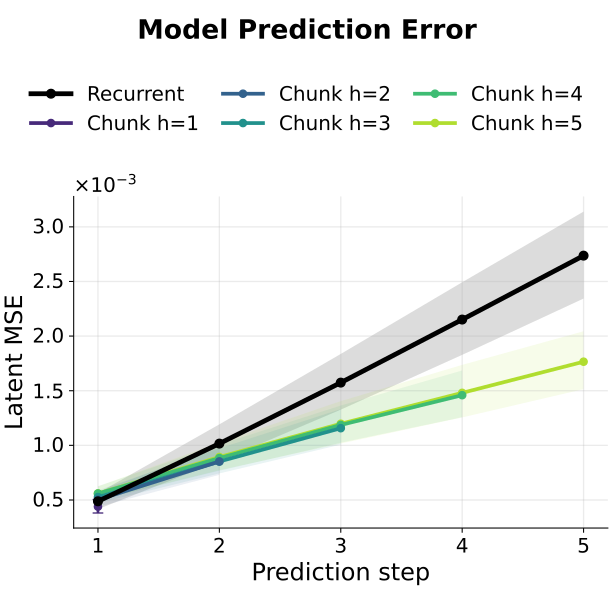
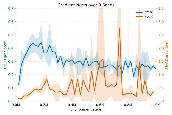
The problem is not limited to computation. A small one-step prediction error becomes part of the next model input, so error can accumulate along the rollout. Policy learning through the trajectory also requires backpropagation through a product of transition Jacobians. Long horizons can amplify the resulting gradient oscillations or make them vanish. CMPO does not avoid future prediction; it changes how the future is represented in the computation graph.
The joint prediction is compact:
$$a_{t:t+H-1}=\pi_\theta(z_t),\qquad z_{t+1:t+H}=f_\phi(z_t,a_{t:t+H-1})$$
The policy maps the current latent state to an action chunk. The dynamics model maps the same current state plus the complete action chunk to all future latent states. Temporal depth still exists in the output tensor, but it no longer requires a sequence of network calls.
2. One call for the entire value expansion
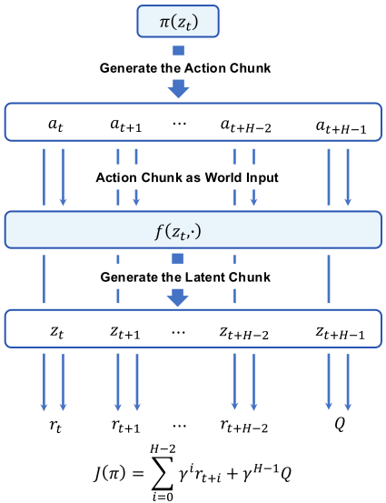
CMPO keeps the standard value-expansion idea: estimate a short-horizon return from predicted rewards and bootstrap from a terminal value. The difference is that the complete rollout is constructed by one forward pass. The reward head supplies intermediate rewards, while an ensemble of Q networks evaluates the terminal state-action pair. The actor is then optimized through this differentiable training-time evaluator.
The paper describes the objective as:
$$\hat G_t^{(H)}=\sum_{k=0}^{H-1}\gamma^k R(z_{t+k},a_{t+k})+\gamma^H Q(z_{t+H},\pi(z_{t+H}))$$
In the public implementation, the utility is slightly shifted. An action chunk contains H actions. Rewards are computed for the first H-1 actions, and the Q function bootstraps from the state-action pair at index H-1:
$$G_t^{(H-1)}=\sum_{k=0}^{H-2}\gamma^kR(z_{t+k},a_{t+k})+\gamma^{H-1}Q(z_{t+H-1},a_{t+H-1})$$
This index mismatch is an implementation detail rather than a second algorithm. It matters when reading the code: the tensor shapes and the paper's terminal-state notation should be checked together instead of inferred separately.
flowchart LR
    O["Observation s_t"] --> ENC["Encoder h"]
    ENC --> LAT["Latent state z_t"]
    LAT --> ACT["Chunk actor π"]
    ACT --> CH["Action chunk a_t ... a_t+H-1"]
    LAT --> DYN["Chunk dynamics f"]
    CH --> DYN
    DYN --> NEXT["Future latents z_t+1 ... z_t+H"]
    NEXT --> RWD["Reward head R"]
    CH --> RWD
    NEXT --> VAL["Critic Q"]
    CH --> VAL
    RWD --> RET["Value-expansion return"]
    VAL --> RET
    RET --> UPD["Actor update"]
3. Error propagation and the pathwise gradient
The motivation section gives a simple error bound. If the local one-step prediction error is at most epsilon and the dynamics model is L_f-Lipschitz with respect to the latent state, the error after k steps is bounded by:
$$\left\|\hat z_{t+k}-z_{t+k}\right\|\le\epsilon\sum_{i=0}^{k-1}L_f^i$$
When L_f is greater than one, the bound grows rapidly with the horizon. A chunk model does not make dynamics prediction exact. It reduces the number of times a prediction must be passed through another network invocation, which removes one source of recursive feedback while retaining a direct multi-step prediction problem.
The recurrent model's policy gradient contains products of transition and policy Jacobians:
$$\frac{d\hat z_{t+k+1}}{d\theta}=\left(\frac{\partial f}{\partial z}+\frac{\partial f}{\partial a}\frac{\partial\pi_\theta}{\partial z}\right)\frac{d\hat z_{t+k}}{d\theta}$$
As the horizon increases, this product can become ill-conditioned. CMPO still needs action derivatives to travel through the world model, but the model parameters can be detached from the policy loss while the action input remains differentiable. That distinction is central to the implementation: the world model is not a black-box target with a fully severed graph; it is a trainable evaluator whose parameter updates and policy gradients are deliberately separated.
4. Model, critic, and policy objectives
The learned components include an encoder, chunk dynamics, reward prediction, a policy, and an ensemble of critics. The model objective combines latent consistency with reward prediction:
$$\mathcal L_{\text{model}}=\mathbb E\left[\sum_{t=0}^{H}\lambda^t\left(\left\|z_t-\operatorname{sg}(h(s_t))\right\|_2^2+\operatorname{CE}(\hat r_t,r_{t+1})\right)\right]$$
The stop-gradient target sg prevents the target latent from being optimized directly. The critic objective applies the same temporal weighting to distributional value errors:
$$\mathcal L_{\text{critics}}=\mathbb E\left[\sum_{t=0}^{H}\lambda^t\operatorname{CE}(\hat q_t,q_t)\right]$$
The actor maximizes the short-horizon return through the chunk model and adds an entropy term:
$$\mathcal L_{\text{policy}}=\mathbb E\left[-\alpha\left(\sum_{i=0}^{H-2}\gamma^iR(z_i,a_i)+\gamma^{H-1}Q(z_{H-1},a_{H-1})\right)-\beta\mathcal H(\pi(\cdot|s))\right]$$
The released configuration uses a consistency coefficient of 20, reward and value coefficients of 0.1, temporal decay rho=0.5, latent and MLP widths of 512, and five Q heads. The high consistency weight is consistent with the paper's argument that reliable latent rollout structure is a prerequisite for a useful value expansion.
| Setting | Value | Role |
|---|---|---|
| Latent width | 512 | Shared representation width for encoder, policy, and dynamics |
| MLP width | 512 | Hidden width for dynamics, reward, actor, and critics |
| Q ensemble | 5 heads | Reduces reliance on a single value estimate |
| Consistency coefficient | 20 | Emphasizes multi-step latent prediction quality |
| Reward / value coefficients | 0.1 / 0.1 | Balance auxiliary prediction and value learning |
| Temporal decay rho | 0.5 | Discounts errors farther into the rollout |
5. What the code actually does
At commit 380ef58, common/world_model.py makes the horizon part of the network dimensions. The dynamics input contains the current latent plus every action in the chunk, and its output contains every future latent. The actor's final dimension is doubled because it predicts both the mean and log standard deviation of the action distribution.
# common/world_model.py:15-26
self._dynamics = layers.mlp(
    cfg.latent_dim + cfg.action_dim * cfg.horizon,
    2 * [cfg.mlp_dim],
    cfg.latent_dim * cfg.horizon,
    act=layers.SimNorm(cfg),
)
self._pi = layers.mlp(
    cfg.latent_dim, 2 * [cfg.mlp_dim], 2 * cfg.action_dim * cfg.horizon
)
The important implementation boundary is the single call to next(). The action chunk is flattened and concatenated with the current latent; the dynamics MLP returns all future states in one invocation. A recurrent implementation would call a one-step model inside a loop. Here the time axis is represented inside the output tensor, not by repeated calls to the same module.
# common/world_model.py:122-127
def next(self, z, a, detach=False):
    """Predicts all horizon latent states from one latent state and action chunk."""
    z = torch.cat([z, a], dim=-1)
    return self._dynamics(z) if not detach else self._detach_dynamics(z)
Despite predicting a chunk, the deployed controller returns only the first action. At every control cycle, act() encodes a new observation, samples a new chunk, and extracts the first element. CMPO therefore reduces inference cost without turning the robot into an open-loop chunk executor.
# cmpo.py:76-86
@torch.no_grad()
def act(self, obs, t0=False, eval_mode=False):
    obs = obs.to(self.device, non_blocking=True).unsqueeze(0)
    z = self.model.encode(obs)
    action, info = self.model.pi(z)
    if eval_mode:
        action = info["mean"][..., : self.cfg.action_dim]
    return action[0][..., : self.cfg.action_dim].cpu(), None
The actor update has a second subtle boundary. It calls _estimate_value(..., detach=True), so model parameters do not accumulate gradients from the policy objective. The action still enters the dynamics model as a differentiable input, allowing pathwise gradients from predicted value back to the actor. Calling this a complete gradient stop would misread the design.
# cmpo.py:170-184
action, info = self.model.pi(zs[0])
chunk_action = action.reshape(
    -1, self.cfg.horizon, self.cfg.action_dim
).permute(1, 0, 2)
# Detached model parameters still propagate gradients through actions.
scores = self._estimate_value(zs[0], chunk_action, detach=True)
self.scale.update(scores)
scores = self.scale(scores)
pi_loss = (-(self.cfg.entropy_coef * info["scaled_entropy"] + scores)).mean()
pi_loss.backward()
6. HumanoidBench evaluation
The simulation study uses 19 HumanoidBench tasks with a Unitree H1hand and a 61-dimensional action space. The tasks span locomotion, terrain traversal, balance, and manipulation. Walking and running test sustained whole-body coordination; stairs, slides, hurdles, mazes, and poles test terrain interaction; door opening, cube manipulation, bookshelf interaction, basketball, window manipulation, and spoon handling require a different kind of precision. The breadth matters because a method that merely accelerates locomotion may not preserve the structure needed for contact-rich control.
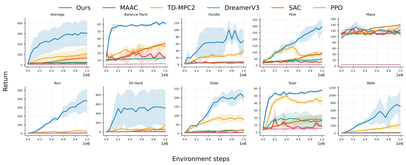
The authors claim stronger average performance and better sample efficiency, not uniform dominance on every task. That is the appropriate reading. Humanoid tasks differ in reward saturation, contact difficulty, and the value of exploration, so a single direct-policy method should not be assumed to win every individual curve.
The wall-time comparison was run on one RTX 4090 for 200,000 steps without Torch Compile. TD-MPC2 took 3.57 hours on Walk and 3.54 hours on Run, while CMPO took 1.74 and 1.72 hours. Per-step inference dropped from 40.8 milliseconds to 1.4 milliseconds on Walk and from 39.5 to 1.3 milliseconds on Run.
| Measurement | Walk / TD-MPC2 | Walk / CMPO | Run / TD-MPC2 | Run / CMPO |
|---|---|---|---|---|
| 200k training steps | 3.57 h | 1.74 h | 3.54 h | 1.72 h |
| One inference step | 40.8 ms | 1.4 ms | 39.5 ms | 1.3 ms |
The training gain is tied to removing recurrent invocation from imagined rollouts. The inference gain also depends on CMPO using a direct actor instead of TD-MPC2's iterative MPPI planning. Those two sources should not be conflated: the reported speedup is a system-level advantage of the complete deployment recipe, not only the cost of one model layer.
7. Ablations expose the real constraint
CMPO requires collaborative chunking. A chunk actor paired with a one-step world model is ill-posed in the paper's framing: the future latent chunk cannot be grounded by a single action. The authors therefore test the opposite mismatch, a chunk policy with a single-step model, to isolate the cost of recurrent model invocation.
| Method | Walk | Run | Stair | Slide |
|---|---|---|---|---|
| CMPO | 954.1 | 629.2 | 60.9 | 265.8 |
| CMPO + MPC | 931.1 | 864.5 | 71.9 | 391.2 |
| Without chunk model | 22.2 | 9.6 | 37.1 | 36.1 |
The largest collapse occurs on Walk and Run, where the method falls from 954.1 and 629.2 to 22.2 and 9.6. Stair and Slide also decline, but by less. This uneven degradation is informative: the pathological effect of recurrent backpropagation depends on task dynamics rather than acting as a universal constant penalty.
Adding MPC improves Run, Stair, and Slide but slightly reduces Walk in this comparison. The paper attributes the gain to MPPI exploration on tasks that have not saturated, while simple tasks already receive enough information from the chunk-model gradient. Chunking and planning are orthogonal choices, so this result should be read as a trade between added test-time computation and exploration.
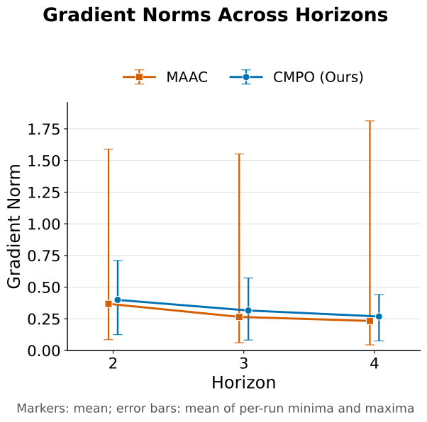
The horizon study is the clearest limitation in the method. CMPO performs best at H=2 and H=4 in the reported sweep. The main experiments use H=3 for a controlled comparison with TD-MPC2. Performance falls when the horizon reaches H=5. Thus the method removes recurrent temporal depth from the network path, but it does not remove the difficulty of predicting a long future directly.
8. Sim-to-real deployment on Unitree Go2
The real-robot experiment trains a bipedal standing and velocity-tracking policy for a Unitree Go2 quadruped. The policy controls all 12 actuated joints through residual joint-position commands tracked by a PD controller. The reward combines linear and angular velocity tracking with base-height, upright-orientation, joint-acceleration, power, collision, action-rate, action-smoothness, and hip-regularization terms.
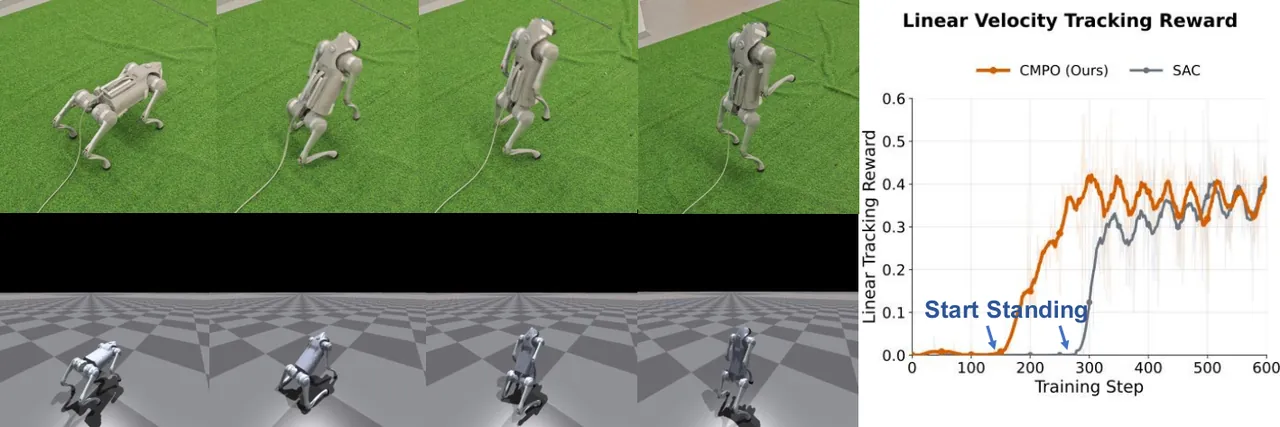
The hardware criterion was to maintain the bipedal posture for 20 seconds. CMPO succeeded in 7 of 10 trials, compared with 4 of 10 for SAC. The authors use SAC because TD-MPC2's iterative planning is not directly compatible with the same low-latency TorchScript feed-forward deployment interface. This is a meaningful engineering result, but it should not be generalized into a claim that CMPO has already beaten every model-based controller on real hardware.
The deployment architecture is arguably the most transferable part of the experiment. Training can use a differentiable multi-step evaluator, while deployment uses a direct policy path without online trajectory sampling. That separation is useful whenever a robot needs fast feedback but the training pipeline can afford richer model-based computation.
9. Limitations and critical assessment
The authors state two limitations directly. First, most of the model architecture is inherited from TD-MPC2; architectures specifically designed for chunk-wise reinforcement learning remain open. Second, executing only the first action preserves responsiveness but discards the remaining actions, which is inefficient in low-dynamic environments. Dynamic execution horizons are therefore identified as an important future direction.
Three additional limitations follow from the evidence. The hardware study contains one task and ten trials per method, so it does not cover different terrains, payloads, or disturbances. The simulation comparison is broad in task count, but a fixed 200,000-step budget leaves open whether the ranking persists after longer training. Finally, direct chunk prediction can reduce recursive depth, but contact discontinuities, distribution shift, and multi-step model bias remain. The decline at horizon five shows that these are not solved by renaming a recurrent rollout as a chunk.
A fair summary is that CMPO makes model-gradient policy optimization shallower and faster. It is well suited to direct feed-forward deployment and can be combined with MPC, but it does not eliminate the fundamental difficulty of learning an accurate long-horizon model.
10. Conclusion
CMPO aligns the temporal granularity of the actor and the world model. A chunk action and a chunk latent rollout are produced together, allowing the value expansion to be evaluated through one model invocation. The design improves training time, inference latency, and gradient stability, with HumanoidBench and Unitree Go2 evidence supporting its practical value. The implementation also makes the boundaries explicit: model parameters are detached from the actor objective while the action path remains differentiable, and deployment executes only the first action to preserve closed-loop control.
The next step is not simply to increase the chunk length. More promising directions are chunk-specific network architectures, adaptive execution horizons, and stronger multi-step consistency under contact changes. The central lesson is concise: CMPO removes the recurrent computation graph, not the need to predict the future.