AgentGarten: Code Worlds for Evolving Agents

AgentGarten: Code Worlds for Evolving Agents
Jiawei Chi, Shangchen Miao, Zhiyuan Shi, Kailu Wu, Hanyang Wang, Weiliang Chen, Qiyu Dai, Jinshan Ren, Jun Gao, Mingsheng Long, Yueqi Duan, Jiangran Lyu, Jialong Wu†, Fangfu Liu† (MirroS / Tsinghua University / Peking University; † project leads)
arXiv:2610.12374v1 [cs.CV], submitted 2026-10-08 · arXiv:2610.12374 · Project page · Code: MirroS-Lab/AgentGarten (Apache-2.0)
Code status: the neural renderer's training recipe (bidirectional → autoregressive → Adversarial Forcing) and its streaming inference server are open, with weights on HuggingFace at MirroS-Lab/AgentGarten-renderer. Two items in the README TODO list are still unchecked: "real-time rendering engine: streaming service and interactive front-end" and "code worlds + agent practice rounds".

In One Sentence

AgentGarten splits an "environment" in half: a simulator or game engine keeps inspectable, editable, persistent state and executes explicit interaction rules, while a single shared neural renderer turns the depth/normal conditions exported by that engine into first-person frames in real time. The renderer is distilled by Adversarial Forcing into a four-step block-causal model that reaches 36.5 fps at 480×832 on one H100. A pretrained agent sees nothing but those generated frames, writes each round of experience into a playbook, and hands it to the next round: shelter-building appears at round 4 of hide-and-seek and ramp-based wall vaulting at round 10, where OpenAI's 2019 self-play RL run needed roughly 25 million and 100 million episodes respectively.

1. The Problem: Simulators and Video World Models Are Each Missing the Other's Half

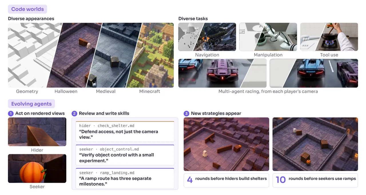
Fig. 1 (paper teaser): the overall claim of AgentGarten. Programmable code worlds on the left, a shared real-time neural renderer on the right, and the two connected only through a structured geometric condition.

Agents learn from action-observation trajectories, so building scalable and generalizable agent capability forces an environment to satisfy two properties that look contradictory at once: faithfulness (preserving the consequences of past actions across long interactions, with consistent state, rules and dynamics) and realism (observations drawn from the real-world visual distribution). The introduction sorts out exactly where each existing route falls short.

Simulators and game engines (Habitat 2.0, ManiSkill2, ProcTHOR) support agent learning with explicit state and programmable interaction rules: state can be queried, rules can be edited, outcomes reproduce. The cost sits on the visual side. Scaling visual diversity means authoring large volumes of 3D assets and building elaborate rendering pipelines, so "creating a new environment" is itself an expensive art-engineering project.

Video world models (Genie, WorldPlay and similar) invert the trade-off: they synthesize rich, interactive visual observations from data, so pixels are not the problem. But the task-relevant state and the physical transition rules live implicitly inside the generation history and the learned representation. You cannot inspect them, edit them, or unit-test them, there is no way to verify that the environment "behaves correctly", and rendering error accumulates straight into the state.

AgentGarten's answer is a division of labour. Every scene program runs inside a simulator or game engine, and the engine owns persistent state plus explicit interaction rules; one shared neural renderer synthesizes the agent's visual observations from the structured conditions the engine exports through a uniform interface. Strict control over state and rules therefore stays in code, and any compatible engine can share the same renderer. New environments can be written by a coding agent from a sentence of text or a single image, then edited and extended entirely in code, with no per-scene visual asset production.

2. Formalizing a Code World: the State Transition Function Never Consumes Rendered Pixels

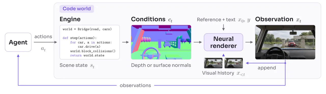
Fig. 2 (paper Fig. 1): interaction and rendering inside a code world. The agent submits actions and receives generated observations; the engine maintains scene state and exports structured conditions (surface normals in the figure); the neural renderer combines those conditions with an appearance reference, text and cached visual history, and the new observation returns to the agent and joins the history.

A code world consists of three things: a scene program $p$, the engine that executes it, and the neural renderer $R_{\theta}$. The program specifies the scene and the interaction rules. Let $s_t$ be the scene state (object poses, articulation, task variables), $\pi_t$ the observing camera pose, and $a_t$ the action of one or more agents. The engine advances state and captures a structured condition $c_t$ from the camera:

$$(s_{t+1},\pi_{t+1}) = f_p(s_t,\pi_t,a_t), \qquad c_t = h_p(s_t,\pi_t) \tag{1}$$

where $f_p$ implements the state transition and $h_p$ renders visible geometry. Given an appearance reference $x_0$ and a text description $y$, the neural renderer generates subsequent observations from the visual history:

$$x_t = R_{\theta}\!\left(x_{{<t}},\ c_{\leq t},\ x_0,\ y\right), \qquad t \geq 1 \tag{2}$$

The agent receives $x_t$, picks $a_t$, and $a_t$ in turn determines the next state and condition through Eq. (1). There is one property here that is easy to read past but is the load-bearing wall of the whole design: no rendered observation appears anywhere in the inputs to $f_p$. The renderer can influence state only through the actions the agent chooses, so rendering error cannot accumulate in the state. The corollary is recording-grade reproducibility: a logged state trajectory can be re-rendered under a different appearance reference or a different camera, and not one word of what actually happened underneath changes. Section 5.1 turns that property directly into a product capability, since the same rollout can be re-shot in another visual style or from another camera position.

Conversely, the renderer can observe state only through $c_{\leq t}$. Attributes the condition does not specify — colour, material, object identity — are given by $x_0$ and $y$ and carried along by the visual history. This also foreshadows the hardest limitation of the system: whatever state the geometric condition fails to encode is simply invisible to the renderer. Section 13 returns to this, using the authors' own §7 example of a bullet spinning about its long axis.

To use a video model as an interactive neural renderer, the paper lists three hard requirements: strictly following the conditions the engine updates, staying visually consistent over long rollouts, and synthesizing observations in fine-grained short blocks so the agent gets feedback immediately after a brief action. The next three sections are the full story of converting a pretrained bidirectional video model into a real-time renderer that meets all three.

flowchart LR
    TASK[Text or a single image] --> CA[Coding agent
writes scene program p and appearance reference x0]
    CA --> ENG[Engine or simulator
persistent state s_t and explicit interaction rules]
    ENG -->|f_p state transition| ENG
    AG[Agent action a_t
submits a short Python program] --> ENG
    ENG -->|h_p exports structured condition c_t
depth or normals at 28 tokens per frame| REND[Shared neural renderer R_theta
Cosmos3-Nano block-causal four steps]
    X0[Appearance reference x0] --> REND
    TXT[Text y] --> REND
    REND -->|480x832 at 36.5 fps| OBS[First-person observation x_t]
    OBS --> AG
    OBS -->|written into a bounded KV cache
5 sink plus 44 recent| REND

3. Structured Conditioning: One Frame of Geometry in 28 Tokens

The chosen condition is a colourized depth map or a surface-normal map. The reasoning is purely engineering: both can be estimated from real video and rendered directly by an engine, and both are three-channel representations, so the pretrained video encoder and Transformer can be reused untouched. Depth for real video comes from ViPE (with Depth Anything 3 as the depth backend) and normals from NormalCrafter; simulated scenes produce both maps straight from geometry, with no need for detailed materials or textures. Each training sample randomly picks one modality.

Depth is encoded with the Vision Banana mapping. Valid depth $d>0$ maps to

$$u(d) = 1 - \left(1 + \frac{\alpha d}{10}\right)^{-2} \tag{14}$$

$\alpha$ is shared across the whole clip: metric depth uses $\alpha=1$; depth of unknown scale first estimates the median $m$ of all valid depths in the clip and sets $\alpha = 10(\sqrt{2}-1)/m$, which places the median at $u=0.5$. Then $u\in[0,1)$ travels once around seven equal-length linear interpolations along the edges of the RGB cube: black, red, yellow, green, cyan, blue, magenta, white, with invalid depth mapped to black. Normals stay in $[-1,1]$ at the autoencoder input, corresponding to the display encoding $(n+1)/2$, and the $x$ component of NormalCrafter's prediction is negated to align with the camera-frame orientation.

The condition tokens are built as

$$G_t = W_{\mathrm{in}}\,\mathcal{P}\!\big([E(S(c))]_t\big) + e_{\mathrm{geo}} \tag{3}$$

$S$ first spatially average-pools the condition video (a factor of 4 per axis, then stretched onto the condition canvas with piecewise-bilinear interpolation), $E$ is the frozen video encoder, $\mathcal{P}$ groups latent patches, and $W_{\mathrm{in}}$ reuses the pretrained RGB input projection directly, plus a zero-initialized modality embedding $e_{\mathrm{geo}}$. Condition tokens carry no diffusion timestep. At the 480×832 output resolution this leaves only 28 condition tokens per latent frame against 390 RGB tokens — roughly a 14× cost difference, which is why conditioning is close to free.

Geometry tokens and RGB tokens are concatenated along the sequence dimension and pass through the same Transformer layers:

$$[\,G_0, G_1, \dots\,]\;[\,R_0, R_1, \dots\,] \tag{4}$$

$R_0$ encodes the appearance reference $x_0$, and the text keys/values are injected through cross-attention. Geometry and RGB share temporal rotary coordinates; spatial coordinates map both grids onto the same image extent, with condition-grid coordinate $u$ aligned by $(u+\tfrac{1}{2})(N_{\mathrm{rgb}}/N_{\mathrm{geo}})-\tfrac{1}{2}$. The paper states explicitly that they use neither channel concatenation nor a ControlNet-style control branch, deliberately avoiding the "pixel-level alignment" inductive bias — only the noisy RGB tokens produce a velocity prediction.

Geometry estimated from real video is not the same as geometry rendered by an engine: there is texture leakage, alignment error and missing observation. To stop the model depending on any one estimator's idiosyncratic cues, training applies a full suite of condition augmentations: randomly keep only depth or only normals, drop both with probability 0.1 (dropped inputs are set to black); suppress texture with probability 0.5 (downsampling factor drawn from $[1.5,3]$, then upsampled back); apply smooth spatial warping anchored at the first frame with probability 0.5 (scale up to 1.15, decaying along the clip); and after encoding, add Gaussian noise of standard deviation 0.4 to the condition latents.

4. Building a World: One Image or One Sentence Yields an Executable Scene Program

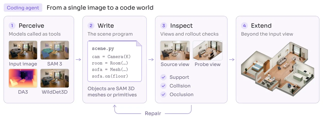
Fig. 3 (paper Fig. 2): a coding agent builds a code world from a single image (living-room example). It calls perception and generation models as tools, uses their outputs to write the scene program, and repairs the program after inspecting rendered views and rollout checks. The extended scene keeps the observed room and adds connected rooms beyond the input field of view as authorial extension; the input image itself supplies the appearance reference $x_0$.

Because appearance is handed entirely to the neural renderer, the scene program needs no detailed materials and no leaf-level assets: coarse geometry is enough as long as it faithfully conveys layout, silhouette, occlusion and motion dynamics. That is the technical basis for the claim that new worlds are cheap.

Building from an image: the input image serves simultaneously as $x_0$ and as the layout reference. Perception and generation models lift the visible content into instance masks, monocular depth with camera intrinsics, 3D bounding boxes and extracted object meshes; the coding agent fits those assets to the estimated geometry, fills unobserved regions with plausible spatial extension, then binds physical properties and interaction rules.

Building from text: the agent writes the scene program directly out of geometric primitives and engine assets, and the first rendered result is passed to an image-editing model to become $x_0$ while preserving the scene layout.

Both routes converge on the same interactive refinement loop: the agent runs test rollouts from several probe cameras, queries the engine's validation interface (contact, collision clearance, occlusion), and iteratively fixes wrong poses, unsupported structures and ambiguous motion before deployment. This is the least "model" part of the paper, yet it decides whether a world is actually usable — an interpenetrating ramp turns every subsequent agent's experience into noise.

5. Three-Stage Training: From a Bidirectional Teacher to a Four-Step Student

The renderer is initialized from the video stream of Cosmos 3-Nano: 36 Transformer layers, hidden width 4096, 32 query heads and 8 key-value heads. The understanding tower (UND) and the generation tower (GEN) are separate; the frozen UND encodes the caption $y$ into per-layer keys/values consumed by GEN, a split that lets the two towers compile and run distributed independently. During distillation the student, teacher and fake-score networks all share the same UND tower and reuse the same caption outputs. The video autoencoder is a frozen Wan VAE (4× temporal, 16× spatial compression), and $2\times2$ patch embedding yields 390 tokens per latent frame at 480×832; the model's temporal grid is handled at 16 fps. A 5-second training window holds 81 frames (1 reference + 20 latent frames = 5 target blocks), and a 15-second window holds 241 frames (reference + 60 latent frames = 15 target blocks). The appearance reference $x_0$ uses the backbone's native clean-frame representation: no diffusion timestep, and it is never denoised.

Training data is RGB video paired with text descriptions, depth and normals: scene captures from DL3DV-10K, driving video from OpenDV, game/navigation/robot-interaction video from the internet, plus a small batch of rendered synthetic scenes whose conditions are exported by the renderer rather than estimated. Every stage runs on 32 H100s with FSDP, one clip per GPU and two-step gradient accumulation, i.e. 64 clips per optimizer update; BF16 compute with FP32 gradient reduction, FP32 parameters for the discriminator head; AdamW everywhere with zero weight decay.

Stage	Parameters updated	Initialization	Learning rate	Adam $(\beta_1,\beta_2)$
1. Geometry conditioning	Self-attention projections and q/k norm; condition embedding	Cosmos 3-Nano	$3\times10^{-5}$	(0.9, 0.99)
2. Causal adaptation, teacher forcing	Same as stage 1	Stage 1	$3\times10^{-5}$	(0.9, 0.99)
3. Distillation: student	Full video stream	Stage 2	$2\times10^{-6}$	(0, 0.999)
3. Distillation: fake score	Full video stream	Stage 1	$4\times10^{-7}$	(0, 0.999)
3. Distillation: discriminator	Head only; backbone is the frozen teacher	Fresh	$2\times10^{-7}$	(0, 0.999)

Table 1 (paper Table 5): three-stage training configuration. Stages 1 and 2 train first on 5-second windows, then on 15-second windows; each distillation stage uses a teacher and fake score matched to the window length. The teacher is the stage-1 model and stays frozen throughout; the text stream and the video autoencoder are frozen for the entire run. Adaptation stages use 100 steps of linear warmup from 10% of the nominal learning rate; distillation stages use a constant learning rate with no warmup.

Stage 2 adapts the geometry-conditioned model into block-level autoregressive generation: latent frames after the reference are cut into fixed-length blocks, each generated from its own aligned geometry plus the already-completed blocks, with no visibility of future blocks. During training the same Transformer holds two copies of every block: a clean copy $P_j$ representing history and a noisy copy $Q_j$ being denoised, each with its own aligned condition tokens. Writing $A_0$ for the reference frame, the attention mask allows

$$P_j \longrightarrow A_0 \cup P_{\leq j}, \qquad Q_j \longrightarrow A_0 \cup P_{{<j}} \cup Q_j \tag{5}$$

Arrows point from a query to the tokens it may read, and text is visible to both. So a noisy copy can read earlier clean blocks and attend bidirectionally within itself, but never sees its own clean target — which lets all target blocks train in parallel, each sampling its own flow time. With $z_j$ the clean latent block and $\mathcal{C}=(x_0,y,c)$ the reference, text and conditions:

$$z_{j,t_j} = (1-t_j)z_j + t_j\epsilon_j, \qquad \mathcal{L}_{\mathrm{TF}} = \mathbf{E}\!\left[\frac{1}{M}\sum_{j=1}^{M}\left\lVert v_{\theta}(z_{j,t_j},t_j \mid z_{{<j}},\mathcal{C}) - (\epsilon_j - z_j)\right\rVert_2^2\right] \tag{6}$$

Each target block holds 4 latent frames, and the reference frame is a separate clean prefix (no timestep, excluded from the loss, never republished after the cache is initialized). To stop the model over-trusting its own history, the visible history of every frame independently receives one of four equally likely perturbations: contrast/exposure scaling about the channel mean (factor drawn from $[0.3,1.7]$), Gaussian noise mixing (strength $[0,1/3]$), bilinear downsampling then upsampling (scale $[0.9,1]$), or nothing at all. The reference frame is never perturbed.

6. Adversarial Forcing, Part I: Distribution Matching on the Model's Own Rollout

Stage 3 distills the teacher-forced model into a few-step renderer trained on its own rollout, and it is made of three pieces: distribution matching against a bidirectional teacher, an exact replay that lets gradients reach the history the model itself wrote, and a real-data adversarial objective with exact R1/R2 regularization.

The first piece follows the Self Forcing DMD route: the student starts from stage 2 and generates each block with a few denoising steps conditioned on its own previous outputs; the frozen stage-1 teacher scores the whole clip jointly; and an auxiliary fake-score model initialized from the teacher learns the student's distribution. Noising the student prediction $\widetilde{z}_{\theta}$ to $y_{\tau}=(1-\tau)\widetilde{z}_{\theta}+\tau\epsilon$, and writing $f_{\mathrm{T}}$ and $f_{\psi}$ for the teacher's and fake-score's clean estimates, the student objective is

$$g = \frac{f_{\psi}(y_{\tau},\tau\mid\mathcal{C}) - f_{\mathrm{T}}(y_{\tau},\tau\mid\mathcal{C})}{a}, \qquad \mathcal{L}_{\mathrm{DMD}} = \mathbf{E}\!\left[\frac{1}{2N}\left\lVert \widetilde{z}_{\theta} - \operatorname{sg}\!\left(\widetilde{z}_{\theta}-g\right)\right\rVert_2^2\right] \tag{7}$$

$a$ is a per-video normalizer, $N$ the number of latent elements, and $\operatorname{sg}$ a stop-gradient; the fake-score model is trained with flow matching on detached student samples. The sampling-trajectory endpoints (normalized flow times) of the four-step renderer are

$$\mathcal{E} = \left(1600/1601,\ 15/16,\ 5/6,\ 5/8,\ 0\right) \tag{15}$$

All blocks in a rollout share this trajectory, and the replay recomputes only its last step. The teacher uses classifier-free guidance scale 6, score times are drawn from a shifted uniform with shift 5, and the fake score takes 5 of its own updates for every 1 student update. Clean estimates are converted from velocity predictions via $f(y_{\tau},\tau) = y_{\tau} - \tau v(y_{\tau},\tau)$. The normalizer is

$$a = \max\!\left\{\operatorname{mean}\left(\left\lvert \widetilde{z}_{\theta} - f_{\mathrm{T}}(y_{\tau},\tau\mid\mathcal{C})\right\rvert\right),\ 10^{-5}\right\} \tag{16}$$

with the mean taken over all latent elements of each video. That $\max\{\cdot,10^{-5}\}$ floor is directly visible in the code: _student_targets in wm/models/dmd.py implements it with clamp_min(1e-5), guarding against the denominator collapsing to zero early in training and blowing up the gradient.

7. Adversarial Forcing, Part II: Exact Replay Puts the History-Writing Forward Pass Back into the Gradient

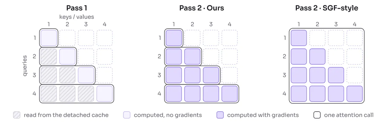
Fig. 4 (paper Fig. 4): exact replay drawn as a block-level attention mask. Row $i$ holds the queries of block $i$, columns the key/value blocks it reads. A rollout runs one attention call per block, reading earlier blocks from a detached cache; this paper's replay runs the same calls but recomputes the history keys/values with gradients, preserving the rollout's execution structure. An SGF-style replay computes the same mask with a single full-sequence call, which changes the numeric execution path.

Standard Self Forcing encodes completed blocks into a detached KV cache. Downstream loss therefore supervises "predictions made from that cache", and not the historical prefill computation that produced those keys and values. Keeping that computation differentiable along a serial rollout would require retaining the entire cache-construction graph linked by the cross-block recursion, at enormous memory cost.

Like Self Gradient Forcing (SGF), this work decouples rollout from gradient propagation with two passes: a first pass rolls out without gradients and records each block's input $U$ at its final denoising time $t^{*}$ together with its clean output $Z$; a second, differentiable replay pass recomputes history and predictions under the visibility pattern of Eq. (5). For block $j$:

$$\widetilde{z}_{\theta,j} = \operatorname{sg}(U_j) - t^{*}\, v_{\theta}\!\left(\operatorname{sg}(U_j),\ t^{*} \mid \operatorname{sg}(Z_{{<j}}),\ \mathcal{C};\ \mathcal{M}_{\mathrm{TF}}\right) \tag{8}$$

The recorded latents stay detached, but their historical encoding is recomputed inside the graph. Downstream loss can then update the parameters that "wrote history into the cache" without differentiating through the sampling trajectory. Both the DMD term and the generator adversarial term use this replayed prediction.

The real contribution is the next sentence. SGF's second pass is implemented with full-sequence FlexAttention: the attention mask matches cached generation, but the kernel, tensor shapes and reduction order do not, so under finite precision the replay can drift away from the sampled trajectory. This paper instead preserves the rollout's execution structure verbatim: attention runs block by block with SDPA, in the same key-value order and with the same call shapes, and projections and feed-forward layers use the same grouping (reference frame first, then per block the condition tokens before the RGB tokens). Grouping matters because projecting an entire packed sequence once and projecting it block by block can round differently, and a trained network amplifies exactly that kind of difference. History keys/values are recomputed and assembled differentiably, so this matched execution preserves the history gradient path. In the implementation the grouping loop lives outside the compiled region while each group's tensor ops stay compiled, so a change in history length or caption length does not trigger re-unrolling and recompilation.

Metric	SGF-style, FlexAttention	This work, block-wise SDPA	Change
Replay error, relative $L_2$	3.99%	0, bitwise identical	—
Forward time	2.95 s	2.79 s	−5.4%
Peak allocated memory	50.83 GiB	50.92 GiB	+0.2%

Table 2 (paper Table 1): replay recomputation error and cost when only the attention execution path changes. One H100, 36 layers, 480×832, 61 latent frames, BF16; times are medians of the replay forward after three warmups and exclude backward and the optimizer update.

"Bitwise identical" is the hardest number in this paper: it makes the replayed prediction and the prediction the rollout actually sampled the same tensor, so the second pass's gradient really is the gradient of the first pass's computation rather than an approximation of it. The cost is close to nothing — the forward is 5.4% faster and memory grows 0.2%. In the implementation each block issues two attention calls: one for its own noisy queries and one for the clean publication that later blocks will read.

The code correspondence is equally direct. The comment in _student_loss in wm/models/dmd.py reads "Pass 2: teacher forcing over the detached Pass-1 queries and context", and the call is self.student.forward_ar(..., clean=rollout.clean) — recomputing with the clean latents recorded in pass 1 as context, exactly Eq. (8). The same function reads back a training-time monitor:

# wm/models/dmd.py
with torch.no_grad():
    recovery = (x0 - rollout.clean).abs().max()
return {**metrics, "metrics/student/sgf_recovery_max_abs": recovery, ...}, loss

sgf_recovery_max_abs is the maximum absolute replay-recovery error, which should be identically zero in theory — it is the watchdog for the "bitwise" claim of Table 2 inside the training logs. The sgf in the name also tells you where this line of work comes from: they kept SGF's two-pass structure and replaced the second pass with an implementation whose execution structure matches.

8. Adversarial Forcing, Part III: Exact R1/R2 Without a Double Backward Through Fused Attention

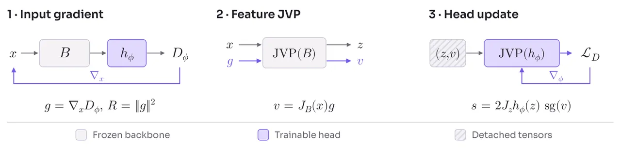
Fig. 5 (paper Fig. 5): exact R1/R2 for a frozen backbone $B$ plus a trainable head $h_{\phi}$. (1) Differentiate only with respect to $x$ to obtain $g$ and $R$; (2) run the backbone's JVP to obtain features $z$ and tangent $v$; (3) run an explicit head JVP on the detached $(z,v)$, returning both the logit and its directional derivative, which yields $s$; a final ordinary backward with respect to $\phi$ updates the head using the full discriminator objective.

Both sides of a pure distribution-matching estimate land on generated samples and are never confronted with real video head-on. Following DMD2, this paper adds an adversarial objective: a trainable head $h_{\phi}$ aggregates intermediate features of the frozen teacher backbone $B$ into a discriminator logit. The backbone is conditioned on geometry and the reference frame, so the discriminator can judge appearance and geometric consistency at the same time. Concretely it reads features after teacher layers 11, 23 and 35; each branch aggregates that layer's tokens with a learned query followed by a residual MLP, and the three branch outputs are concatenated into a single logit.

The adversarial pairing uses R3GAN's relativistic form. Let $r$ and $f$ be the logits for a real clip and a student prediction (both noised identically, at the same timestep, under the same conditions):

$$\mathcal{L}_{\mathrm{G}} = \mathbf{E}\!\left[\operatorname{softplus}\!\left(\operatorname{sg}(r) - f\right)\right], \qquad \mathcal{L}_{\mathrm{rel}} = \mathbf{E}\!\left[\operatorname{softplus}(f - r)\right] \tag{9}$$

The student minimizes $\mathcal{L}_{\mathrm{DMD}}+\lambda_{\mathrm{G}}\mathcal{L}_{\mathrm{G}}$. The generator-side gradient is injected into the second pass's graph through a linear surrogate: with $h=\partial\mathcal{L}_{\mathrm{G}}/\partial\widetilde{z}_{\theta}$ (critic parameters fixed), it enters the student graph as $\langle \widetilde{z}_{\theta}, \operatorname{sg}(h)\rangle$, so both the adversarial and the DMD objectives act through the replay without retaining the rollout graph. In code this is the single line loss = loss + (x0 * gan_gradient).sum().

The difficulty is the regularization. R3GAN constrains the discriminator with R1 and R2, the squared input-gradient norms on real and generated samples:

$$D_{\phi}(x) = h_{\phi}(B(x)), \quad R_1 = \mathbf{E}_{x\sim p_{\mathrm{data}}}\lVert \nabla_x D_{\phi}(x)\rVert_2^2, \quad R_2 = \mathbf{E}_{x\sim p_{\theta}}\lVert \nabla_x D_{\phi}(x)\rVert_2^2 \tag{10}$$

Their parameter gradients normally require "differentiating through a backward". Fused attention kernels inside the backbone (FlashAttention and friends) do not support that double backward. APT's workaround approximates R1 with random perturbations. This paper instead computes the exact penalty and the exact head-parameter gradient, and it can do so because of one fact: the backbone is frozen.

For a single sample, write $z=B(x)$, $A=J_B(x)$ and $u=\nabla_z h_{\phi}(z)$. Then

$$g = A^{\top}u, \qquad R = g^{\top}g, \qquad v = Ag \tag{11}$$

$g$ comes from one vector-Jacobian product (a parameter-frozen backward through the head, then through the backbone), and $v$ from one Jacobian-vector product that pushes $g$ forward through the frozen backbone carrying no gradient graph. Neither step materializes $A$. Because neither $z$ nor $A$ depends on $\phi$:

$$\nabla_{\phi} R = 2\left(\frac{\partial u}{\partial \phi}\right)^{\!\top} v = \nabla_{\phi}\!\left[\,2\,J_z h_{\phi}(z)\,\operatorname{sg}(v)\,\right] \tag{12}$$

The right-hand side is the gradient of a directional derivative that belongs to the head alone, computable by writing the head's JVP out of ordinary differentiable ops (Appendix B). With $s = 2J_z h_{\phi}(z)\operatorname{sg}(v)$, the surrogate

$$\widetilde{R} = \operatorname{sg}\!\left(\lVert g\rVert_2^2\right) + s - \operatorname{sg}(s) \tag{13}$$

evaluates to the true penalty while having an exact first-order derivative with respect to $\phi$. The discriminator then minimizes $\lambda_{\mathrm{D}}\big(\mathcal{L}_{\mathrm{rel}}+\tfrac{\gamma}{2}(\widetilde{R}_1+\widetilde{R}_2)\big)$. The detached features $z$ and tangents $v$ of real and generated samples pass through the head once and produce both the relativistic logit and the directional term; one ordinary backward updates the head. No step differentiates through a backward kernel, and there are no finite differences and no random directions.

This derivation lives in the repository at wm/models/exact_regularization.py::exact_penalties, whose three comment blocks map almost line for line onto Eq. (11)–(13):

# wm/models/exact_regularization.py
# 1. Input gradient through the frozen backbone and a frozen head.
leaf = rows.detach().requires_grad_(True)
with frozen_parameters(head), torch.enable_grad():
    (direction,) = torch.autograd.grad(head([features(leaf)]).sum(), leaf)
direction = direction.detach()
# 2. Feature tangents along that gradient (forward mode, no graph).
with torch.no_grad(), fwAD.dual_level():
    dual = features(fwAD.make_dual(rows.detach(), direction.to(rows.dtype)))
...
# 3. Head directional derivative, differentiable w.r.t. the head only.
return ExactPenalty(logits=logits, penalty=penalty,
                    surrogate=surrogate - surrogate.detach())

Step 1's torch.autograd.grad is $g=A^{\top}u$ (a VJP); step 2's fwAD.make_dual under no_grad is $v=Ag$ (a forward-mode JVP carrying no graph); step 3 does the double differentiation with create_graph=True over the small head only. That last line, surrogate - surrogate.detach(), is the literal implementation of Eq. (13): value zero, gradient exactly $\mathrm{d}R/\mathrm{d}\phi$. The config wm/configs/experiments/cosmos3/dmd_gan_exact.py sets exact_regularization_weight to 0.075, with an adjacent comment reading "0.075 = 30 * 0.05^2 matches the local scale of the finite-difference recipe" — that is, they deliberately matched the strength of the exact version to the local scale of an APT-style finite-difference recipe so the comparison is apples to apples.

flowchart TD
    S2[Stage 2 teacher-forced model] --> P1[Pass 1 rollout without gradients
four denoising steps per block writes a detached KV cache
records input U and clean output Z]
    P1 --> P2[Pass 2 differentiable replay
block-wise SDPA keeps the same KV order and call shapes
recomputes history K V under the Eq 5 visibility pattern]
    P2 --> DMD[Distribution matching DMD
fake score minus teacher score divided by normalizer a]
    P2 --> GAN[Generator adversarial term
relativistic softplus pairing
gradient injected into the replay graph through a linear surrogate]
    DMD --> STU[Student update at learning rate 2e-6]
    GAN --> STU
    TEA[Frozen teacher backbone features after layers 11 23 35] --> HEAD[Discriminator head
learned query pooling plus residual MLP]
    HEAD --> PEN[Exact R1 R2
one VJP yields g and one forward-mode JVP yields v
surrogate value equals the true penalty with an exact first-order derivative]
    PEN --> DISC[Discriminator update at learning rate 2e-7
one ordinary backward and no double backward]

9. Streaming Inference: Sink Prefix, Sliding Window, Hand-Written Kernels

At inference the renderer first prefills the reference frame and the text, then denoises each arriving block and commits the clean prediction into a bounded KV cache. The cache holds a permanent sink prefix (starting with $x_0$) and a sliding window over recent history, with older frames evicted; the current block attends to all cached frames plus text, and once denoising finishes the clean block joins the recent window. The measured configuration is 5 sink frames plus 44 recent latent frames (one of the history windows used during distillation) plus the 4 current frames, so each block attends over 49 frames of history.

What happens when a rollout exceeds the training horizon? The paper uses a top-aligned rotary position remapping: the active block is clamped at the horizon boundary, recent history is shifted to sit before it and re-rotated, which preserves relative temporal distances while the geometric condition keeps following the true simulation timeline. The code is wm/kernels/stream_cache.py::relocate — the function name says exactly what it does.

Transformer execution over short blocks is dominated by memory bandwidth and kernel-launch overhead. Rather than relying on torch.compile (cold-start compilation takes minutes), they write custom Triton kernels that fuse the elementwise operators around attention (RMSNorm, RoPE rotation, gated activation), removing intermediate memory round-trips; fixed-shape blocks use CUDA graph capture/replay to eliminate host-side launch overhead (wm/inference/serving.py::_GraphCall); and during real-time serving the standard VAE decoder can optionally be swapped for a distilled tiny decoder that reconstructs pixel frames within 10 ms, running in FP16. In interactive deployment the engine pushes conditions to a GPU worker, and decoded frames stream to the agent or a browser over WebRTC with bounded queueing delay.

Anatomy of one 16-frame served block, one H100, BF16	Time	Share
Condition encoding	10.6 ms	2.4%
Transformer: four denoising steps + cache publication	414.4 ms	94.4%
Tiny decoder and host transfer	8.8 ms	2.0%
Total wall clock	438.8 ms	—
Throughput	36.5 frames/s	—

Table 3 (paper Table 2): steady-state inference cost. The cache holds 5 sink plus 44 recent latent frames with 4 current latent frames, combined with hand-written kernels, CUDA graphs and the tiny decoder. Stage times are medians of GPU time; the total is the mean wall clock per block and includes work beyond the three stages. Measurements come from blocks 17–48 of a 48-block, 769-frame rollout, averaged over two rollouts; attention is dense. The share column is computed here against 438.8 ms.

What this table is worth staring at is how it lays out the cost structure of a "real-time video world model": 94% of the time goes to the Transformer's four denoising steps and cache publication, while condition encoding and decoding together take under 5%. The 28-token condition design really is almost free, and any remaining speedup has to come from attention and step count — four steps is already very few, and 49 frames of history is already window-truncated. Against a 16 fps temporal grid, 36.5 fps is about 2.3× real-time headroom, and that headroom is exactly what a scenario like "two agents in one world, each needing its own first-person stream" consumes (the racing column of paper Fig. 8 shows two agents sharing one world state).

10. The Code-World Library and Round-Based Practice

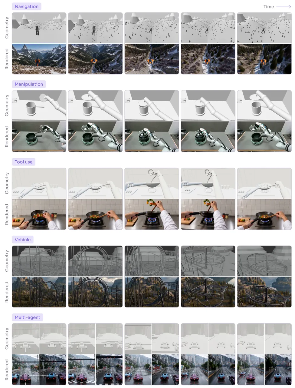
Fig. 6 (paper Fig. 8): five code worlds, five moments from one rollout each. Within a column, the top row is untextured scene geometry and the bottom row is the generated observation it conditions. The racing group contains first-person views of two agents sharing one world state. Scene programs write only coarse geometry; appearance is supplied by the renderer from the initial image, text and visual history.

Different scene programs plus compatible engines make up code worlds that share one renderer. The examples given cover navigation, manipulation, tool use and multi-agent interaction. Interactive deployment adds browser games whose rules live entirely in code: bowling, a penalty shootout, and a crate-vault puzzle — the player's keyboard, mouse or gamepad input advances the code world, and the rendered stream is its only view. Because state evolution is explicit it can also be replayed and re-rendered: a recorded rollout can be re-shot in another visual style or from another camera position, and nothing that happened changes at all.

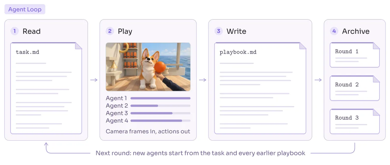
Fig. 7 (paper Fig. 10): one practice round. The agent reads a task file (goal, available actions and constraints, but no solution), plays in parallel within a fixed budget, sees only camera frames, and writes a playbook at the end. Playbooks are archived, and the next round's agent starts a fresh conversation from the task file plus every playbook so far.

Hide-and-seek is only one instance of this general procedure. Practice proceeds in rounds: a round starts from a task file stating the goal, the available actions and the constraints, but not a solution. One or more agents play in parallel, each with a fixed step or simulation-time budget. They see the world only through camera frames synthesized by the neural renderer: no coordinates, no map, no score before the episode ends. Afterwards each agent writes a playbook recording what it tried, what it observed, what it still suspects, and what it wants to verify next. Playbooks are archived, and the next round's agent launches in a fresh conversation with the task file and every playbook from previous rounds.

This "rounds plus playbooks" structure is nothing like a policy gradient in reinforcement learning: what gets updated is the context, not the weights. Its readability is also completely different — what one round learns is a piece of Markdown a human can read, edit and delete, rather than a parameter delta whose semantics you cannot diff. The cost is just as clear: a playbook belongs to one world and is short enough to read in full, so once there are many worlds someone has to decide which lessons to keep, which to merge and which to throw away.

11. Hide-and-Seek Revisited: 4 Rounds Against 25 Million Episodes

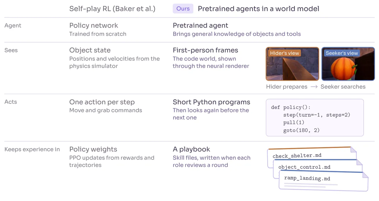
Fig. 8 (paper Fig. 9): hide-and-seek under two settings. Top: self-play reinforcement learning trains a policy network on object state and reward. Here a pretrained agent watches first-person frames from the neural renderer, acts by submitting short Python programs, and stores what it learns in skill files inside a playbook. Bottom: three episodes from the recorded experiments, seen from an overhead camera.

In OpenAI's 2019 hide-and-seek study, agents trained with self-play reinforcement learning developed shelter building, ramp use, and defensive counter-strategies against those tools: the paper reports shelter building emerging after roughly 25 million episodes and seeker ramp use another 75 million episodes later (about 100 million in total). Those agents observed object state. This work revisits the same setting with a pretrained agent that can reason about "what just happened" and modify how it behaves, and that sees the world only through the renderer.

The setting is a sequential single-hider, single-seeker variant: the hider arranges the scene first, then hands control to the seeker. Each agent receives first-person observations generated by the neural renderer from the environment's structured conditions, acts by submitting short Python programs for movement and object interaction, and then observes the resulting change through the renderer. It gets no object coordinates, no hidden world state and no private observations of its opponent.

Each role maintains its own playbook, organized as a library of skill files: Markdown notes that may contain code, one lesson per file. The recorded experiments start from an empty playbook and run several rounds of five episodes each, on sampled layouts and seeds. At the end of every round each role reviews its action programs and the visual evidence it is allowed to see, identifies failures, and adds skill files to the playbook. The next round's agent receives the accumulated skills, interprets the current scene, and judges which old experience is relevant. Both successful and failed attempts feed subsequent revisions.

Three characteristic behaviours appear during interaction (Fig. 8): the hider moves a panel to rebuild a shelter; the seeker carries a ramp to the inner wall and climbs over it; and the seeker's first jump falls short, so it moves the ramp closer to the wall and tries again. These three episodes are direct evidence that multi-step physical tool-use strategies can be acquired and refined purely from neurally rendered first-person observation — the third especially, since it contains a failure diagnosis and a correction of a geometric parameter.

Strategy	Self-play RL, 2019 training episodes	This work's pretrained visual agent rounds
Building a shelter	about 25 million	4
Using a ramp to enter a shelter	about 100 million	10

Table 4 (paper Table 3): physical tool-use milestones under the two paradigms. Five episodes per round, so round 4 is about 20 episodes and round 10 about 50.

The paper is deliberately restrained about how to read this table, and its reasoning is worth restating: the two numbers reflect two fundamentally different learning paradigms, not a sample-efficiency ratio. The 2019 agents learned physical dynamics and competitive coordination from random weights, operating directly on ground-truth coordinate state; a foundation-model agent already holds abstract knowledge about objects, tools and geometry from web-scale pretraining. Its main challenge is not discovering concepts from scratch but grounding abstract knowledge into closed-loop sensorimotor action, diagnosing spatial execution failures from synthetic visual observation alone with no access to state, and refining tactical execution across rounds.

12. Round-by-Round Results in Four Worlds

The same procedure is carried into four more worlds, changing only the world and its task file, with four rounds each. Companion dog: keep a dog willingly engaged (reaching out, petting, playing with a ball) during a 60-second session. Single-lane bridge: two cars, each driven by one agent from a windshield view, must swap ends as fast as possible over a bridge that fits one car. Herding: two dogs that see the world only from their own eye height must drive four sheep into a pen and hold them for five seconds. Quarry loader: a wheeled loader must push two rocks onto a staging platform within 360 seconds, deliver one of them into a hopper behind a wall, then park. In all four worlds the agents act directly on first-person observations synthesized by the neural renderer in real time, with no access to internal simulation state or the engine's raw geometry buffers.

World	Metric	Round 1	Round 2	Round 3	Round 4
Companion dog	Interaction score	13	14	19	19
Single-lane bridge	Seconds until both cars arrive, lower is better	71	68	45	41
Herding	Score out of 100	60	90.1	87.6	88.3
Herding	Sheep penned, out of 4	3	4	4	4
Quarry loader	Score out of 100	30	0	30	90.9

Table 5 (paper Table 4): results per round in the four worlds. Each row is that world's own terminal metric, one episode per round.

The four curves do not have the same shape, and that is more informative than "everything improved". The companion dog climbs from 13 to 19 and then stays at 19; the single-lane bridge descends monotonically 71→68→45→41 and is the only clean learning curve; herding times out in round 1 (3 of 4 sheep penned), pens all 4 in every later round, and its score wobbles slightly around 88. The loader is the most telling: round 1 clears the rocks but makes no further progress for 30 points, round 2 scores 0, round 3 is back to 30, and round 4 clears the rocks, feeds the hopper and parks, using 329 of the 360 seconds for 90.9.

That zero should not be read as noise. Each round is a single episode with no multi-seed variance, so every step of these curves can be pushed around by the luck of one run; and round 2's collapse to zero shows precisely that an inherited playbook can also lead an agent astray — a written-down lesson influenced the next round's judgement without ever being verified. The authors have in fact already identified the antidote in §7: because a code world can be reset and replayed exactly, a lesson can be tested before it is passed on. That step is not part of these experiments yet.

13. Limitations

(Author-stated, §7) The geometric condition is redundant, and redundancy costs detail. Once an object's shape is known, its rigid motion needs only a few pose parameters, yet the condition video repeats those surfaces across many pixels and frames. Spatial downsampling saves cost but removes the thin structures, narrow gaps and small contact changes that fine control needs.

(Author-stated, §7) State the geometry does not specify is state the renderer cannot know. A rotationally symmetric object can spin about its axis while depth and normals do not change at all, even though a marking painted on it is turning; material, colour and object identity are likewise not determined by geometry. Visual history can preserve these attributes but may lose them after long occlusion or a revisit beyond the memory window. The direction the authors propose is a more abstract, compact condition interface, such as structured text describing object properties and interaction state (which could state the orientation and angular velocity of a bullet spinning about its long axis even when the depth and normal maps are unchanged), or high-dimensional latent features. The interface also determines which worlds cannot be presented at all: a geometry-only renderer cannot tell a spinning wheel from a stationary one, so tasks depending on that kind of state are out of reach today.

(Author-stated, §7) Worlds are authored one at a time. "Generating a world is the easy part"; the hard part is deciding whether it deserves an agent's time: can the task be solved from what the agent can see, will a careless policy fail, and is there a lesson that carries into the next round. The authors want those checks to run automatically before any agent practises in a new world. There is a scale problem on the experience side too: the playbooks here belong to a single world and are short enough to read in full, so across many worlds an agent must decide which lessons to keep, merge or discard, and find the few that apply to the scene in front of it.

(Our judgement) Render quality is compared qualitatively only, with no numeric metric. Section 4.1 uses Fig. 7 to show 30-second rollouts side by side: Self Forcing develops repeated surface texture and loses scene detail over time, while Adversarial Forcing keeps natural texture. The conclusion rests entirely on the eye — the main text reports no FVD, no LPIPS, and no reference to a user study. For a paper arguing that the renderer can serve as an agent's eyes, this is the piece of evidence most worth adding: how much of an agent's failure comes from rendering distortion currently cannot be attributed.

(Our judgement) The agent-side evidence is not reproducible and is statistically thin. The repository open-sources renderer training and inference, but "code worlds and agent practice rounds" is still unchecked in the README TODO, so none of Section 5's results can be re-run today. Meanwhile Tables 4 and 5 use one episode per round with no multiple seeds and no confidence intervals; and the 25-million-episodes-versus-4-rounds comparison in Table 4, which the authors explicitly say is not a sample-efficiency ratio, is still the pair of numbers most likely to be quoted with that premise stripped away.

(Our judgement) The "bitwise identical" guarantee has boundaries. The zero error in Table 2 holds when replay and rollout use the same execution structure, and training does run that way (sgf_recovery_max_abs is watching it). But online serving takes a different path through CUDA graphs plus the tiny decoder, and in a multi-agent world the batching of two first-person streams may differ from the grouping used in training. The paper reports no replay consistency for the serving path, so the guarantee should be read as "history gradients are exact during training", not "every deployment configuration is bitwise reproducible".

14. Takeaways and What Comes Next

The skeleton of this technical report is a clean separation of duties: state to the engine, pixels to the renderer. On the engine side is an explicit world that can be inspected, edited and replayed exactly; on the renderer side is a video model converted into a block-causal, four-step, 36.5 fps generator, held up by two engineering contributions inside Adversarial Forcing — exact replay puts history encoding into the gradient and aligns it bitwise, and exact R1/R2 keeps discriminator regularization exact on top of fused attention. The two sides are joined only by a narrow interface of 28 geometric tokens, so any compatible engine can share this one renderer and the cost of a new world drops to "write some coarse geometry code".

The most valuable empirical evidence it offers is not 36.5 fps but this: a pretrained agent watching only rendered frames can ground web-scale abstract tool knowledge into closed-loop physical execution within a handful of rounds — together with the round mechanism that externalizes experience into readable text. This route does not compete with self-play RL: one accumulates experience in weights, the other in context; the former needs tens of millions of episodes, the latter tens of episodes but bounded by the priors the base model already has.

Looking forward, three intermediate steps are the ones worth watching. First, replace the dense geometric video condition with structured text or latents so that state like "the wheel is spinning" becomes visible — this decides the boundary of which worlds can be built at all. Second, let coding agents author worlds automatically and run the "is this worth practising in" admission checks automatically. Third, add a verification step to playbooks: since a code world can be reset and replayed exactly, a lesson can perfectly well be tested once before it is handed to the next round. None of the three has results yet, but the paper explains clearly why each one is hard.

Golden Quote

Generating a world is the easy part. The harder question is whether it deserves an agent's time: can the task be solved from what the agent can see, will a careless policy fail, and is there a lesson that carries into the next round?