ID Balancing: Stable Training of Extremely Sparse MoE via PID-Based Load Control

ID Balancing: Stable Training of Extremely Sparse MoE via PID-Based Load Control
Peng Jin*, Zihan Qiu*, Zekun Wang*, Bo Zheng* (equal contribution), Yang Xu, Tian Xie, Xiao Li, Huaqing Zhang, Haoran Lian, Rui Men, Dayiheng Liu (corresponding)
Qwen Team, Alibaba Token Hub, Alibaba Group · arXiv:2609.39137v1 [cs.LG], 2026-09-30 · arXiv page
Code status: no official implementation released as of v1. The closest public work is torchtitan PR #1197, which experiments with router biases using Kimi K3's Quantile Balancing as a baseline, and Marin's validation of Quantile Balancing at 32B-A5B; neither implements ID Balancing. The method-to-equation mapping below follows the arXiv v1 full text and Algorithm 1.

In one sentence

Read auxiliary-loss-free MoE load balancing as control: DeepSeek's loss-free method is a fixed-step integral controller (it only sees the sign of the error), Kimi K3's Quantile Balancing is a generalized proportional controller (it only chases a target computed from the current batch), and both are half a controller. ID Balancing supplies the missing halves with a magnitude-aware integral term plus a derivative term gated on worsening imbalance: under Top-3-of-768 routing it cuts worst-case backbone MaxVio from 31.11 to 15.33 and training-average MinVio by more than 12%, and as total parameters grow from 18.9B to 69.9B its worst MaxVio stays essentially flat at roughly 89.6% below the auxiliary-loss baseline, with no loss in language-modeling or downstream quality.

1. The problem: sparsity is the throttle, load imbalance is the brake pad

The scaling logic of MoE is clean: each token activates only $K$ of $E$ experts, so with $K$ fixed, adding experts adds capacity without adding per-token compute, and pushing the active fraction $K/E$ lower becomes the natural scaling direction. But the sparser the routing, the more a small perturbation of router scores near the Top-$K$ boundary rewrites token assignments, and the more sensitive expert loads become. Overloaded experts slow MoE computation (the slowest rank sets the all-to-all step time); underloaded experts receive no training signal, which leaves purchased parameters idle. The first attacks training efficiency, the second attacks parameter utilization, and together they produce "more experts, no more capability".

The paper quantifies this along two axes: sparser routing and larger models. Figure 1(a)(b) compares Top-10, Top-5 and Top-3 of 768 experts on the same 18.9B architecture trained for 120B tokens: worst backbone MaxVio climbs from 16.42 (auxiliary loss, Top-10) to 211.19 (DeepSeek loss-free, Top-3), with training-average MinVio rising in lockstep. Figure 1(c) fixes Top-10-of-768 and scales total parameters from 18.9B to 69.9B: the auxiliary-loss worst MaxVio jumps from 16.42 to 75.03 while ID Balancing moves only from 8.36 to 7.79. Load control is not a nice-to-have metric here; it is the precondition for scaling sparse MoE further.

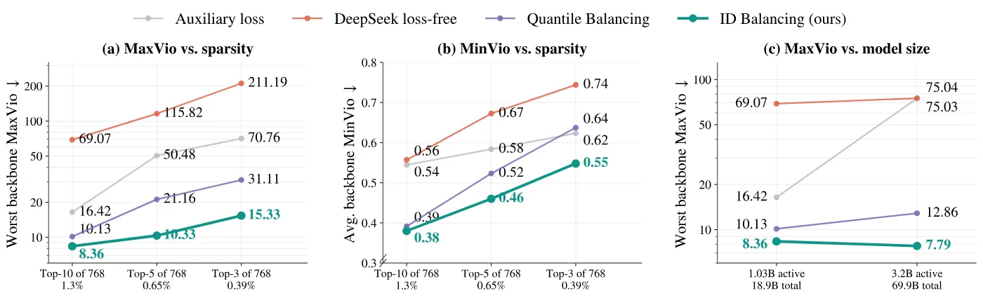
Figure 1 (paper Fig. 1): load control degrades with sparsity and with scale. (a)(b) Worst backbone MaxVio and training-average backbone MinVio for Top-10/5/3 of 768 on the 18.9B model; (c) worst MaxVio under fixed Top-10-of-768 as total parameters grow from 18.9B to 69.9B. ID Balancing is the flattest curve on both axes.

All existing auxiliary-loss-free methods share one mechanism: a non-trainable bias per expert, added to router scores for Top-$K$ selection but excluded from the combination weights. They differ only in how the bias is updated. The paper's first contribution is reading this family of updates through a single PID frame, where the bias is the controller state and the deviation from uniform load is the feedback signal. The reading yields a blunt conclusion: DeepSeek's loss-free method has only an integral term with a fixed step, and Quantile Balancing has only a proportional term with no memory. Both are incomplete PID controllers, and whatever ailment an incomplete controller has in control theory, they have here.

2. The control view: three updates, three incomplete controllers

2.1 The three PID branches

The standard discrete-time PID form responds to the current error (proportional), accumulates past errors (integral), and reacts to changes in the error (derivative):

$$u_{t}=\underbrace{K_{p}\,e_{t}}_{\text{proportional}}+\underbrace{K_{i}\sum_{\tau\leq t}e_{\tau}}_{\text{integral}}+\underbrace{K_{d}\,(e_{t}-e_{t-1})}_{\text{derivative}} \tag{1}$$

Eq. 1 is linear in the error. The paper explicitly adopts a generalized PID view: it keeps the temporal roles of the three branches (current / accumulated / change) but allows nonlinear transformations of the feedback. This matters, because the "proportional" branch of Quantile Balancing is not a linear $K_p e_t$ at all; it is a target computed from the batch score distribution. Without the generalization the unifying view would not stand.

2.2 Load balancing as a control loop

An MoE layer has $E$ routed experts and a Top-$K$ router. A token representation $\mathbf{x}$ yields logits $\mathbf{z}=W_r\mathbf{x}$, and an activation $\sigma$ gives expert scores $s_i=\sigma(z_i)$. Loss-free methods keep a non-trainable bias $b_i$ per expert and select

$$\mathcal{T}(\mathbf{x})=\operatorname{TopK}_{i\in[E]}\left(s_{i}+b_{i}\right) \tag{2}$$

Combination weights normalize only the original scores $s_i$, so the bias affects who is selected but not how they are weighted. Let $n_i^{(t)}$ be the tokens assigned to expert $i$ at step $t$; the uniform target and normalized load error are

$$\bar{n}^{(t)}=\frac{1}{E}\sum_{i=1}^{E}n_{i}^{(t)},\qquad e_{i}^{(t)}=\frac{\bar{n}^{(t)}-n_{i}^{(t)}}{\bar{n}^{(t)}} \tag{3}$$

Negative error means overload, positive error means underload, and the loop closes: the bias vector $\mathbf{b}^{(t)}$ is both the persistent controller state and the control input to the next Top-$K$ decision; the token-count vector $\mathbf{n}^{(t)}$ is the measured output; each step updates the bias from $\mathbf{e}^{(t)}$, rewriting routing and loads at the next step. The two deviations are measured by

$$\mathrm{MaxVio}^{(t)}=\frac{\max_{i}n_{i}^{(t)}-\bar{n}^{(t)}}{\bar{n}^{(t)}},\qquad \mathrm{MinVio}^{(t)}=\frac{\bar{n}^{(t)}-\min_{i}n_{i}^{(t)}}{\bar{n}^{(t)}} \tag{13}$$

MaxVio is bounded above by $E/K-1$ (all tokens into one expert); MinVio lies in $[0,1]$ and reaches 1 when some expert receives no token at all. Every load judgment in the paper reduces to these two numbers: Last1k and Avg. are means over the final 1k steps and the full window, backbone values average over 20 layers, and Worst MaxVio takes the maximum over layers and steps.

2.3 Placing the baselines into the position form

Writing the proportional, integral and derivative contributions as $\mathbf{P}^{(t)},\mathbf{I}^{(t)},\mathbf{D}^{(t)}$, the position-form update is

$$\mathbf{b}^{(t+1)}=\mathbf{P}^{(t)}+\mathbf{I}^{(t)}+\mathbf{D}^{(t)} \tag{4}$$

DeepSeek loss-free is fixed-step integral control. The update adds the sign of the error times a step size, which telescopes into a running sum of signs:

$$\mathbf{b}^{(t+1)}=\mathbf{b}^{(t)}+\eta\,\operatorname{sign}(\mathbf{e}^{(t)})=\eta\sum_{\tau\leq t}\operatorname{sign}(\mathbf{e}^{(\tau)})=\mathbf{I}^{(t)} \tag{5}$$

The sign throws away error magnitude: an error of 0.01 and an error of 5 receive the same correction $\eta$. Large errors are therefore under-served (the early mean-MaxVio spike of 132 in Figure 2(a) is its signature), while near balance the same step overshoots. As a side effect, $\sum_i \operatorname{sign}(e_i)$ is generally nonzero, so the common bias component drifts.

Quantile Balancing is generalized proportional control. It accumulates no history; instead it computes a target bias from the current batch's score distribution and jumps straight to it. Let $\mathbf{S}^{(t)}$ hold the scores of $m$ tokens over $E$ experts and let $\alpha_i^{(t)}$ be the $(K+1)$-th largest biased score of token $i$, i.e. the current cutoff. The target is a quantile of score margins:

$$\mathcal{Q}_{j}=-\operatorname{quantile}_{1-K/E}\left(\left\{S_{i,j}^{(t)}-\alpha_{i}^{(t)}\right\}_{i=1}^{m}\right),\qquad \mathbf{b}^{(t+1)}=\mathcal{Q}(\mathbf{S}^{(t)},\mathbf{b}^{(t)})=\mathbf{P}^{(t)} \tag{7}$$

The target places roughly a $K/E$ fraction of biased margins above zero, matching the desired load $q=mK/E$; at scale the quantile is estimated from a per-expert margin histogram. It depends on the current bias through $\alpha_i$, so it retains state dependence, but it does not explicitly accumulate past load errors, which is why it lands in the nonlinear proportional branch. The price is that the target moves with the batch score distribution: the paper's EMA diagnostic shows larger late-stage bias drift, and smoothing that drift away simultaneously weakens early load control. You cannot have both.

Auxiliary loss is outside this family. It adds the product of routed fraction and mean router probability to the objective and updates the router weights $W_r$ through gradients:

$$\mathcal{L}_{\text{aux}}=\alpha\sum_{i=1}^{E}f_{i}P_{i},\quad f_{i}=\frac{1}{T}\sum_{\mathbf{x}}\mathbb{1}[i\in\mathcal{T}(\mathbf{x})],\quad P_{i}=\frac{1}{T}\sum_{\mathbf{x}}p_{i}(\mathbf{x}) \tag{8}$$

It shares one optimization process with the language-modeling objective, so the two objectives trade off against each other, and no control bias is maintained. The high-learning-rate stress test makes the trade-off concrete: raising $\alpha$ from 0.05 to 0.5 does not restore balance; it pushes LM loss to about 2.45, mean MaxVio above 50 and MinVio to 1.0, and both runs terminate before 30k steps.

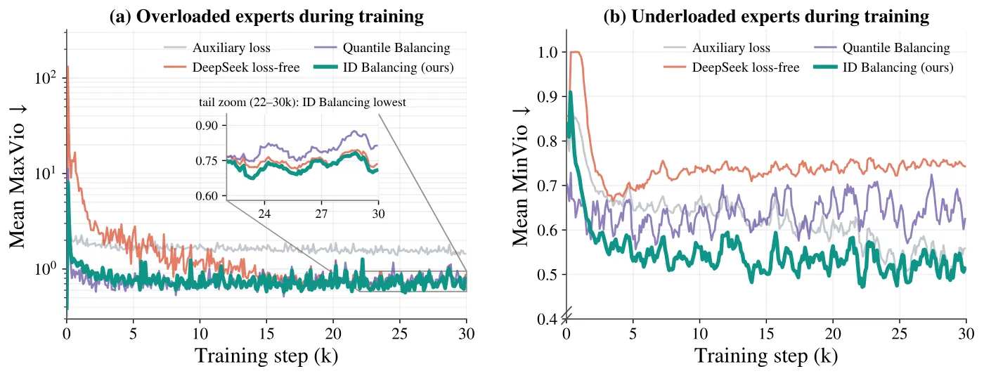
Figure 2 (paper Fig. 2): Top-3-of-768, 18.9B, 120B tokens, averaged over 20 backbone layers. (a) Mean MaxVio on a log scale; (b) mean MinVio. DeepSeek's early overload spike and the sustained underload of auxiliary loss and DeepSeek are the typical symptoms of the two incomplete controllers; ID Balancing ends with the lowest training-average underload.

3. ID Balancing: integral sees magnitude, derivative sees worsening

The control view prescribes exactly one sentence: corrections should scale with the load error and respond when the imbalance worsens. ID Balancing is that sentence implemented as two terms plus a re-centering step. It changes only the bias update; routing stays Eq. 2 and the error stays Eq. 3.

3.1 Magnitude-aware integral term

Replace the sign with the error itself:

$$b_{i}^{(t+1)}=b_{i}^{(t)}+K_{i}\,e_{i}^{(t)} \tag{9}$$

The correction grows with $|e_i|$ and shrinks as the expert approaches its target load, and because the bias accumulates these corrections the memory of integral control is retained. A side benefit the paper calls out: since $\sum_i e_i^{(t)}=0$ by Eq. 3, the integral update preserves a zero-mean bias when started from $\mathbf{b}^{(0)}=\mathbf{0}$, a property the fixed-sign update lacks. Figure 3 compares the two integral updates under Top-3-of-768: magnitude scaling lowers the worst-layer MaxVio peak and the sustained underload, i.e. stronger early correction and better expert utilization.

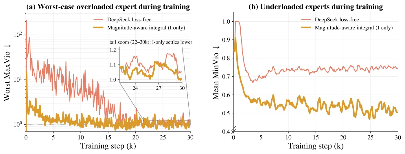
Figure 3 (paper Fig. 3): magnitude-aware integral control versus DeepSeek's fixed-step integral (18.9B, Top-3-of-768, 120B tokens). (a) Worst MaxVio across the 20 layers, log scale; (b) mean MinVio. Bigger error, bigger correction removes the fixed step's early under-response.

3.2 Worsening-gated derivative term

The integral sees magnitude but cannot tell a growing error from a shrinking one of the same size. Add the error change

$$\Delta e_{i}^{(t)}=e_{i}^{(t)}-e_{i}^{(t-1)},\quad e_{i}^{(-1)}=0 \tag{10}$$

and keep only the changes that push an existing imbalance farther from zero:

$$g_{i}^{(t)}=\mathbb{1}\left[e_{i}^{(t-1)}\,\Delta e_{i}^{(t)}>0\right] \tag{11}$$

The gate opens when the previous error and its change share a sign, i.e. the imbalance keeps growing without crossing zero; it stays closed when the error is unchanged, moves toward zero, or crosses zero, and it is closed at the first step. The correction $K_d g_i \Delta e_i$ accumulates in the bias alongside the integral term. Its input is an error difference, but unlike a classical derivative output it is both gated and accumulated: a brake assist that engages only while things get worse. Figure 4(a) shows the active-gate fraction falling from about 0.38 early to about 0.25 late, so the derivative term retires itself as worsening events become rare; Figures 4(b)(c) show lower early overload and a lower share of tokens routed to the busiest 10% of experts, with trajectories converging back to the integral-only curve later.

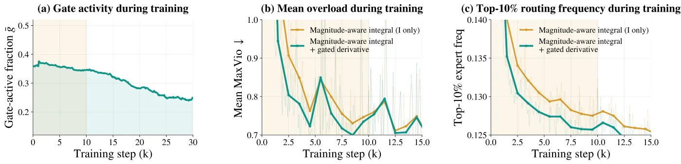
Figure 4 (paper Fig. 4): the operating window of the gated derivative. (a) Active-gate fraction averaged over 20 layers, from about 0.38 to about 0.25; (b) mean MaxVio; (c) share of tokens routed to the busiest 10% of experts (balanced target 0.10). The derivative term does its work early.

3.3 Why no proportional term, and why re-center

ID Balancing sets $K_p=0$. The reason is not saving one computation: a proportional term (in the generalized sense, i.e. Quantile's chase of a batch-computed target) makes the bias jump with the batch score distribution, perturbing the Top-$K$ boundary repeatedly and producing larger late-stage bias drift. Smaller changes in relative biases mean less perturbation of routing, and smoother bias trajectories are also friendlier to weight merging such as checkpoint averaging, where merged weights must stay compatible with the routing state of the sources. The paper's EMA diagnostic, applied only to Quantile, confirms the trade-off is real: smoothing suppresses drift but weakens early load control. ID Balancing gets low drift and good balance from the integral plus gated derivative, with no extra smoothing.

The closing step removes the common component. The integral term is zero-mean, but the gated derivative sum $\sum_i g_i \Delta e_i$ generally is not, so the bias mean can drift. Adding the same constant to every expert bias changes neither score rankings nor $\mathcal{T}(\mathbf{x})$, so each update simply subtracts the mean:

$$\widetilde{b}_{i}^{(t+1)}=b_{i}^{(t)}+K_{i}e_{i}^{(t)}+K_{d}g_{i}^{(t)}\Delta e_{i}^{(t)},\qquad b_{i}^{(t+1)}=\widetilde{b}_{i}^{(t+1)}-\frac{1}{E}\sum_{j=1}^{E}\widetilde{b}_{j}^{(t+1)} \tag{12}$$

Note that re-centering removes only the common drift; it does not bound the differences between expert biases, so all control authority still comes from the error feedback. The whole method needs only $\mathcal{O}(E)$ token-count feedback per layer and adds no balancing gradient to the language-modeling objective. Algorithm 1 in full:

flowchart TD
    A[Route batch with frozen bias
TopK of s_i + b_i per Eq.2] --> B[Count tokens per expert n_i
over microbatches and DP group]
    B --> C[Uniform target n_bar
and normalized error e_i per Eq.3]
    C --> D{Worsening gate open?
e_prev and delta_e same sign}
    D -->|yes| E[Add gated derivative
K_d times delta_e]
    D -->|no| F[Skip derivative term]
    E --> G[Add magnitude-aware integral
K_i times e_i]
    F --> G
    G --> H[Re-center bias to zero mean
ranking unchanged]
    H --> I[Store e_prev and route next step]
    I --> A

4. Experiments: four stress directions

4.1 Main comparison: sparsity

The main runs use the Qwen-3.8-Next hybrid architecture: 20 Transformer layers (one full-attention layer every four, gated linear attention elsewhere), 768 routed experts plus 1 shared expert per MoE layer, and one MTP module; 18.9B total parameters with 0.87 / 0.91 / 1.03B active for Top-3 / 5 / 10. Training uses 120B tokens, global batch 1024, peak learning rate 2.54e-3 with cosine decay to 3e-5, and all methods are compared over the same 30k-step window. Baseline settings: DeepSeek $\eta=0.001$, auxiliary loss $\alpha=0.05$, Quantile with its original update and no EMA, ID Balancing $K_i=K_d=6\times10^{-3}$.

Method	Act./Total	LM loss	MaxVio Last1k	MaxVio Avg.	MaxVio Worst	MinVio Last1k	MinVio Avg.
Top-3 of 768, 120B tokens
Auxiliary loss	0.87B / 18.9B	1.7527	1.4809	1.7239	70.76	0.5462	0.6232
DeepSeek loss-free		1.7426	0.7314	1.9356	211.19	0.7487	0.7441
Quantile Balancing		1.7432	0.8093	0.7985	31.11	0.6504	0.6373
ID Balancing		1.7426	0.7026	0.7931	15.33	0.5266	0.5480
Top-5 of 768, 120B tokens
Auxiliary loss	0.91B / 18.9B	1.7378	1.0296	1.2925	50.48	0.4537	0.5836
DeepSeek loss-free		1.7280	0.5821	1.4814	115.82	0.6741	0.6725
Quantile Balancing		1.7303	0.6376	0.6394	21.16	0.5335	0.5232
ID Balancing		1.7299	0.5404	0.6498	10.33	0.4238	0.4601
Top-10 of 768, 120B tokens
Auxiliary loss	1.03B / 18.9B	1.7180	0.6862	1.0342	16.42	0.3631	0.5446
DeepSeek loss-free		1.7121	0.4418	0.9715	69.07	0.5534	0.5571
Quantile Balancing		1.7133	0.4776	0.4832	10.13	0.4060	0.3914
ID Balancing		1.7118	0.3863	0.5110	8.36	0.3282	0.3800

Table 1 (paper Tab. 1, backbone part): 18.9B, 120B tokens, one shared 30k-step window. Last1k and Avg. average over 20 layers; Worst is the maximum over layers and steps. The three bias-based methods differ in LM loss by at most 0.0023, while their load metrics differ by an order of magnitude.

Three readings. First, LM loss is nearly a tie: auxiliary loss is worst in every block but by no more than 0.0023 against the bias family, so the load-control gains are not bought with language-modeling quality or with balancing gradients in the objective. Second, the gap between methods widens with sparsity: Worst MaxVio in the Top-10 block is 16.42 / 69.07 / 10.13 / 8.36, and in the Top-3 block it becomes 70.76 / 211.19 / 31.11 / 15.33, with DeepSeek's fixed step losing control by two orders of magnitude at extreme sparsity. Third, ID and Quantile divide the labor rather than dominate each other: ID takes Worst and Last1k MaxVio plus Last1k and Avg. MinVio in all three blocks, while Quantile keeps the lower Avg. MaxVio in Top-5 and Top-10 (0.6394 vs 0.6498, 0.4832 vs 0.5110). ID wins on worst case and underload; Quantile wins on mid-to-late average overload.

4.2 Scale and learning rate

On scale: fixing Top-10-of-768 and growing total parameters from 18.9B to 69.9B (1.03B to 3.2B active), ID's worst backbone MaxVio moves from 8.36 to 7.79, essentially unchanged and about 89.6% below the auxiliary-loss baseline in the same block. This is the most scaling-relevant figure in the paper (Figure 1(c)): within this configuration family, the difficulty of load control does not grow with size.

On learning rate: the Top-10-of-768 model is trained for 120B tokens at a constant 5.86e-3, i.e. 2.3x the standard peak. In Table 2, ID and Quantile post Last1k backbone MaxVio of 0.6437 and 0.5021 against 3.1383 and 1.3755 for auxiliary loss and DeepSeek; ID also takes the lowest LM loss (2.0007) and the lowest MTP Last1k / Avg. MaxVio (0.4642 / 0.5068). On the auxiliary-loss side, raising $\alpha$ only makes things worse: at $\alpha=0.5$ the LM loss reaches about 2.45, mean MaxVio exceeds 50, MinVio hits 1.0, and the runs die before 30k steps. When balancing gradients share one optimizer with language-modeling gradients, that trade-off breaks first at high learning rate.

Method	LM loss	bb MaxVio Last1k	bb MaxVio Avg.	bb MaxVio Worst	bb MinVio Last1k	bb MinVio Avg.	MTP MaxVio Last1k	MTP MaxVio Avg.	MTP MaxVio Worst
Auxiliary loss	2.0099	3.1383	2.8379	20.89	0.8423	0.8458	3.5640	3.0533	4.83
DeepSeek loss-free	2.0031	1.3755	1.7811	72.54	0.8730	0.8269	0.5033	0.7124	17.98
Quantile Balancing	2.0009	0.5021	0.4979	2.96	0.4083	0.3938	0.6243	0.5836	10.77
ID Balancing	2.0007	0.6437	0.7274	11.97	0.4828	0.4950	0.4642	0.5068	7.20

Table 2 (paper Tab. 3): 1.03B-active / 18.9B-total, Top-10-of-768, constant learning rate at 2.3x peak. Quantile holds the tightest backbone balance; ID holds the best LM loss and MTP balance; the two gradient-based baselines lose control across the board.

4.3 Continued pretraining: shrink the gains by 1000x

DeepSeek freezes expert biases during continued pretraining, which avoids routing perturbation from bias updates but also switches off active load correction; as the model adapts to a new data distribution, loads drift while the bias stays put. The paper's answer is to scale $K_i,K_d$ from 6e-3 down to 6e-6, a factor of 1000. On two 28-layer models with Top-8-of-256 and Top-10-of-768 routing, the frozen bias settles at mean MaxVio 2.2 to 2.5 (MinVio about 0.83) and 6 to 7 (MinVio about 0.95, severe expert underuse), while the reduced gains keep LM loss within 0.001 of the frozen baseline over the second half of continued pretraining and bring mean MaxVio to about 1 and from about 6 down to 1.4. Reduced gains are the default for continued pretraining: active correction stays on without disturbing adaptation. The DeepSeek and Quantile baselines keep their biases frozen in this stage.

4.4 Downstream quality and inference-time utilization

Models trained for 560B tokens are evaluated on nine benchmarks: MMLU / MMLU-Pro / SuperGPQA for knowledge, MATH / GSM8K for math, BBH for reasoning, MMMLU for multilingual understanding, and EvalPlus plus MultiPL-E for code. In the Top-8-of-256 block ID averages 55.81, the best of the four; in the Top-10-of-768 block ID reaches 58.66 against 58.12 for auxiliary loss and beats that baseline on five of nine benchmarks. The margins are noise-level, but the direction is consistent: the load-control gains cost no capability.

Method	MMLU	MMLU-Pro	SuperGPQA	MATH	GSM8K	BBH	MMMLU	EvalPlus	MultiPL-E	Avg.
Top-8 of 256, 3.0B / 24.8B, 560B tokens
Auxiliary loss	68.00	47.10	27.36	47.12	74.94	69.57	59.82	51.51	46.22	54.63
DeepSeek loss-free	70.08	47.23	27.43	45.84	76.54	71.09	60.61	53.96	46.66	55.49
Quantile Balancing	70.49	48.06	27.61	48.54	74.37	69.94	60.17	52.27	42.46	54.88
ID Balancing	69.58	48.19	27.52	47.92	74.49	72.91	60.78	56.48	44.40	55.81
Top-10 of 768, 3.2B / 69.9B, 560B tokens
Auxiliary loss	71.67	50.91	30.15	50.74	79.08	71.09	63.62	56.55	49.28	58.12
DeepSeek loss-free	72.02	50.11	30.10	50.72	77.37	72.47	64.07	57.65	51.52	58.45
Quantile Balancing	72.37	51.14	30.40	50.86	75.40	73.42	64.13	57.94	51.41	58.56
ID Balancing	72.09	51.46	29.95	50.30	78.17	73.96	63.58	56.90	51.52	58.66

Table 3 (paper Tab. 2): downstream nine benchmarks at 560B tokens; block headers give active / total parameters. ID posts the best or tied-best average in both sparsity blocks.

Inference-time utilization is measured on the continued-pretrained models by recording per-layer loads and router scores in prefill mode over the nine benchmarks. Under Top-8-of-256 the inactive-expert ratio is 3.1% for ID against 3.5% (DeepSeek), 4.1% (Quantile) and 4.7% (auxiliary loss); under Top-10-of-768 ID cuts the average ratio from 8.4% to 6.4% and the first-layer ratio from 9.3% to 2.6% relative to auxiliary loss. This is consistent with the lower training-time MinVio: what is fed evenly during training is used fully at inference. The top-$K$ gating-score entropy and the full-pool selection-score entropy (Figure 6, panels b, c, e, f) differ little among the three loss-free methods, so ID's gain lives in which experts get selected, not in how evenly the selected mixture is weighted.

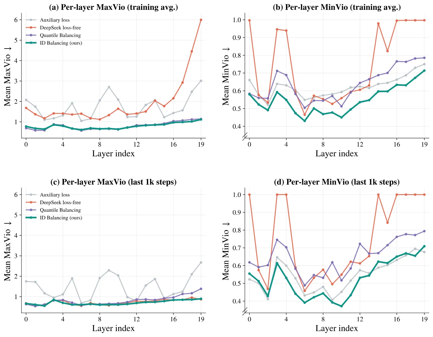
Figure 5 (paper Fig. 10): per-layer MaxVio / MinVio over the 20 backbone layers under Top-3-of-768; top row training average, bottom row final 1k steps. DeepSeek's training-average overload reaches about 6.0 at layer 19 while its last-1k value is 0.9; MinVio rises with depth for all four methods, a trend ID lowers but does not eliminate.

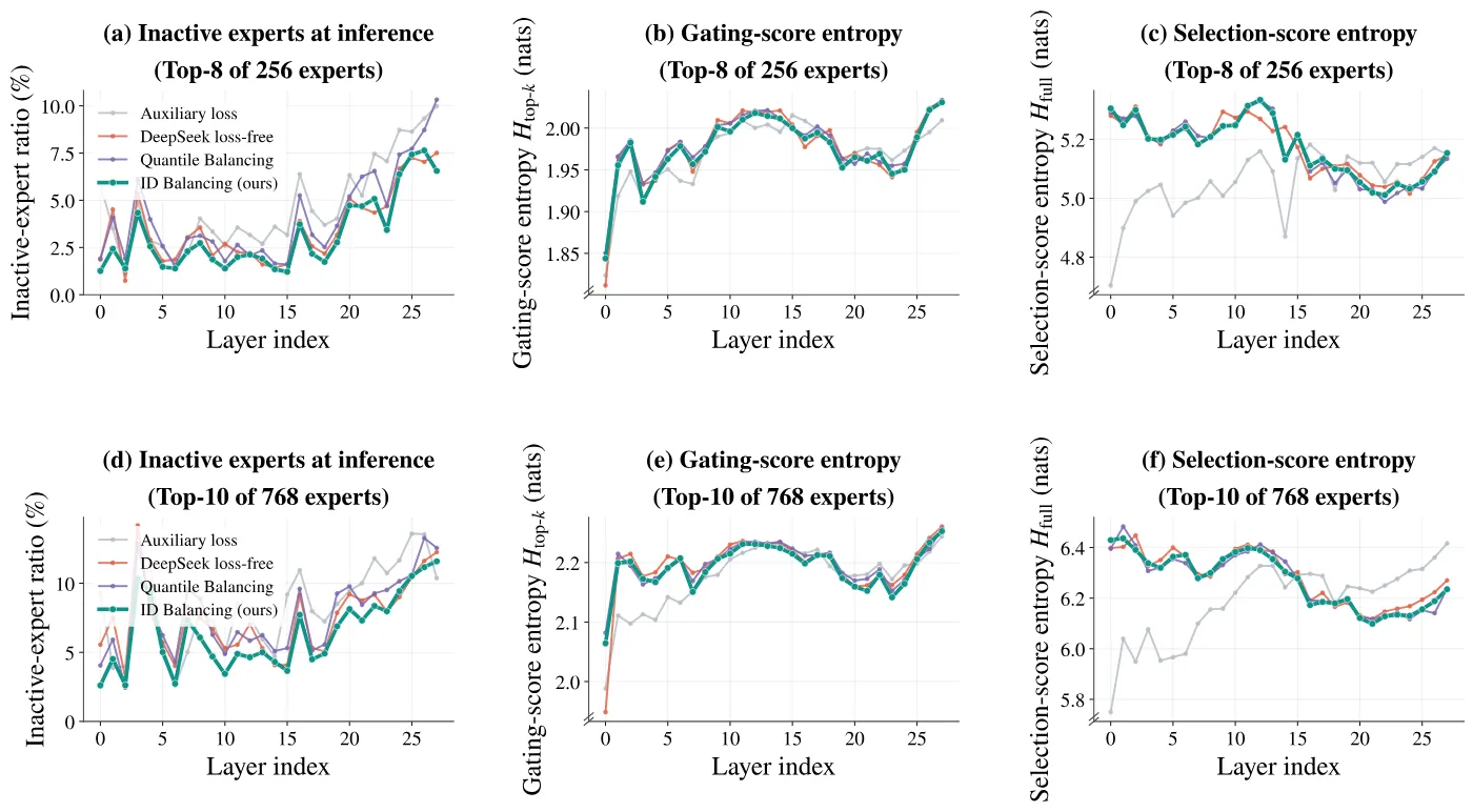
Figure 6 (paper Fig. 11): inference-time expert utilization. (a,d) Inactive-expert ratio; (b,e) top-K gating-score entropy; (c,f) full-pool selection-score entropy. Top row Top-8-of-256, bottom row Top-10-of-768.

4.5 Ablations: how the two gains were chosen

With $K_d=0$ and $K_i\in\{3,6,9\}\times10^{-3}$: 3e-3 corrects early imbalance slowly; 6e-3 lowers training-average backbone MaxVio from 0.9459 to 0.8003 and worst from 23.26 to 14.96; 9e-3 improves the average only marginally (0.7872) but pushes worst backbone MaxVio back up to 20.13 and worst MTP MaxVio from 15.18 to 35.56. With $K_i=6\times10^{-3}$ and $K_d\in\{0,3,6,12\}\times10^{-3}$: the derivative improves early backbone control (mean MaxVio from 2.0020 to 1.9330 over steps 0-1k, and from 0.9059 to 0.8612 over 1-5k) and cuts the sampled cumulative excess above layer-mean MaxVio 1 by 57.9% over 1-5k relative to the integral-only baseline; the price is MTP overload rising with $K_d$ (training-average MTP MaxVio 0.8862 to 0.9698 to 1.0922). The default $K_i=K_d=6\times10^{-3}$ sits at the intersection: strong enough early backbone control, MTP cost not yet out of hand, and the best LM loss and training-average backbone MinVio among the tested gains.

Integral gain ($K_d=0$)	LM loss	bb MaxVio Last1k	bb MaxVio Avg.	bb MaxVio Worst	bb MinVio Avg.	MTP MaxVio Worst
$K_i=3\times10^{-3}$	1.7422	0.6759	0.9459	23.26	0.5777	9.14
$K_i=6\times10^{-3}$	1.7431	0.6924	0.8003	14.96	0.5527	15.18
$K_i=9\times10^{-3}$	1.7429	0.6831	0.7872	20.13	0.5436	35.56

Table 4 (paper Tab. 4): 0.87B-active / 18.9B-total, Top-3-of-768, 30k steps. The integral optimum is 6e-3; beyond it the MTP module and the worst case start paying.

Derivative gain ($K_i=6\times10^{-3}$)	LM loss	0-1k MaxVio	1-5k MaxVio	Avg. MaxVio	Avg. MinVio	MTP Avg. MaxVio
$K_d=0$ (integral only)	1.7431	2.0020	0.9059	0.8003	0.5527	0.8862
$K_d=3\times10^{-3}$	1.7428	1.8900	0.8869	0.7910	0.5485	0.9459
$K_d=6\times10^{-3}$	1.7426	1.9330	0.8612	0.7931	0.5480	0.9698
$K_d=12\times10^{-3}$	1.7427	1.8100	0.8131	0.7812	0.5501	1.0922

Table 5 (paper Tab. 5): the derivative buys early backbone control and pays in MTP overload. The default 6e-3 balances the two.

5. Limitations

Author-stated, first: the evaluation covers several routing sparsities, model sizes and training conditions within a family of decoder-only MoE models with fixed Top-$K$ routing; extending it to other architectures and routing schemes (expert choice, hash layers) is left as future work.

Author-stated, second: the accumulated worsening-gated derivative update is supported empirically. The paper provides ablations and trajectories but no argument for why it should beat a non-accumulated derivative term or other gate forms; what the gated accumulation corresponds to in control-theoretic terms (some anti-windup flavor, presumably) is never developed.

Author-stated, third: the scaling experiments compare complete configurations that differ in depth, width, active and total parameters and training duration, so they assess load control across configurations without isolating model size alone. The "size-invariant" reading of Figure 1(c) is an observation within a configuration family, not a scaling law.

My fourth: ID and Quantile divide the labor rather than dominate, but the abstract's narrative leans toward domination. In Table 1, Quantile holds the lower Avg. backbone MaxVio in Top-5 and Top-10; in Table 2's high-learning-rate block Quantile's backbone Last1k is 0.5021 against ID's 0.6437; and on the MTP side ID trails repeatedly (Table 1 Top-3 MTP Worst 33.42 vs 30.89). If your concern is mid-to-late average overload or MTP-module balance, Quantile remains the stronger choice, and that is not visible from the abstract.

My fifth: the gains come from a coarse hand-tuned grid (3 to 4 points each) shared across all sparsities, with no adaptive or per-layer gain mechanism, even though Figure 5 shows layer-wise imbalance profiles differ strongly (MinVio rises systematically with depth). Per-layer gains are an obvious unexplored direction. The paper also reports no wall-clock, throughput or system-cost numbers, so the $\mathcal{O}(E)$ feedback advantage stays at the level of complexity notation and engineers must estimate it themselves.

6. Summary and outlook

ID Balancing contributes on three levels. The first is a view: unifying auxiliary-loss-free balancing as PID turns DeepSeek into fixed-step integral control and Quantile into generalized proportional control, converting each method's ailment (under-response to large errors / no memory of past errors) into a known failure mode of control theory instead of two isolated empirical observations. The second is a method: magnitude-aware integral plus worsening-gated derivative plus zero-mean re-centering, needing only $\mathcal{O}(E)$ token counts per layer and no balancing gradient, i.e. almost free to implement. The third is evidence: stress tests along sparsity, scale, learning rate and continued pretraining all hold, with LM loss and downstream scores intact.

For practitioners pretraining MoE models the actionable takeaways are concrete: at extreme sparsity, first check whether your controller's integral step scales with the error; during continued pretraining, do not freeze the bias, drop the gains by three orders of magnitude; when sweeping gains, track the MTP module's balance separately because its optimum does not coincide with the backbone's. For control theorists this is a rare case of classical controller design intuition transferred directly onto deep-learning training stability and winning: the gated derivative is a conditionally accumulated correction that deserves a rigorous analysis, and deserves to be tried on balancing problems beyond routers.

Golden quote

Corrections should scale with the load error and respond when the imbalance worsens.