PAPER DEEP DIVE
GS3LAM: Gaussian Semantic Splatting SLAM
Recently, the multi-modal fusion of RGB, depth, and semantics has shown great potential in dense Simultaneous Localization and Mapping (SLAM). However, a prerequisite for generating consistent semantic maps is the availability of dense, efficient, and scalable scene representations. Existing semantic SLAM systems based on explicit representations are often limited by resolution and an inability to predict unknown areas. Conversely, implicit representations typically rely on time-consuming ray tracing, failing to meet real-time requirements. Fortunately, 3D Gaussian Splatting (3DGS) has emerged as a promising representation that combines the efficiency of point-based methods with the continuity of geometric structures. To this end, we propose GS3LAM, a Gaussian Semantic Splatting SLAM framework that processes multimodal data to render consistent, dense semantic maps in real-time. GS3LAM models the scene as a Semantic Gaussian Field (SG-Field) and jointly optimizes camera poses and the field via multimodal error constraints. Furthermore, a Depth-adaptive Scale Regularization (DSR) scheme is introduced to resolve misalignments between scale-invariant Gaussians and geometric surfaces. To mitigate catastrophic forgetting, we propose a Random Sampling-based Keyframe Mapping (RSKM) strategy, which demonstrates superior performance over common local covisibility optimization methods. Extensive experiments on benchmark datasets show that GS3LAM achieves increased tracking robustness, superior rendering quality, and enhanced semantic precision compared to state-of-the-art methods. Source code is available at https://github.com/lif314/GS3LAM.
One-Sentence Summary
GS³LAM stores color, depth, opacity, covariance, and a low-dimensional semantic feature in every Gaussian, then uses one differentiable splatting pipeline for real-time rendering, camera tracking, and dense semantic mapping while two additional constraints control geometric degradation and incremental forgetting.
Why Dense Semantic SLAM Is Hard
A useful indoor robot map must do more than localize the camera. Navigation, manipulation, and human-robot interaction all need spatial labels: which surface is a wall, which region is a table, and where a free floor corridor begins. Classical semantic SLAM systems often attach labels to points, voxels, surfels, or meshes. These representations are easy to update locally, but their resolution is tied to explicit storage. They also struggle to interpolate across unobserved space and rarely provide a single differentiable path from sensor observations to appearance, geometry, and semantics.
Neural radiance fields offer a continuous alternative. An implicit field can synthesize novel views and add semantic output channels, but volumetric rendering requires many ray samples per pixel. That cost conflicts with the frame-by-frame operating pattern of SLAM, where tracking, mapping, and visualization all compete for the same compute budget. High offline rendering quality is not enough if the map cannot keep pace with the camera.
Three-dimensional Gaussian splatting sits between an explicit point cloud and a continuous neural field. Each primitive has a position, orientation, anisotropic scale, opacity, and color. When projected to the image plane, primitives are sorted and composed with alpha blending. The representation preserves the locality and editability of points while allowing ellipsoids to cover surfaces smoothly. GS³LAM exploits this middle ground and turns the Gaussian cloud into a multimodal map.
A naive extension would store a one-hot class vector in every Gaussian. That makes per-primitive storage grow with the class count and forces the rasterizer to carry high-dimensional semantic payloads. A separate two-dimensional segmentation network would avoid that cost but could produce labels that are not tied to the reconstructed 3D surface. The paper instead learns a compact feature per Gaussian, renders it through the same alpha weights as RGB and depth, and applies a shared lightweight decoder at the image level.
Two incremental-mapping failures remain. New Gaussians are initialized from depth, so their scales can vary sharply across frames; overly large primitives blur object boundaries, while tiny primitives leave holes. In addition, local covisibility sampling can repeatedly optimize a small set of neighboring views while starving older or weakly connected regions. The resulting field forgets previous viewpoints even though every local frame may look acceptable during its own update.
Technical Background
Let the scene contain $N$ semantic Gaussians. Primitive $i$ has mean $\boldsymbol{\mu}_i$, covariance $\boldsymbol{\Sigma}_i$, opacity $o_i$, RGB color $\mathbf{c}_i$, and semantic feature $\mathbf{f}_i$. The covariance is factored through a rotation matrix $\mathbf{R}_i$ and a scale matrix $\mathbf{S}_i$. This parameterization keeps the matrix positive semidefinite and gives each ellipsoid an interpretable orientation and extent.
$$ \mathcal{G}:=\{(\boldsymbol{\mu}_i,\boldsymbol{\Sigma}_i,o_i,\mathbf{c}_i,\mathbf{f}_i)\mid i=1,\ldots,N\} $$
$$ \boldsymbol{\Sigma}_i=\mathbf{R}_i\mathbf{S}_i\mathbf{S}_i^{T}\mathbf{R}_i^{T} $$
For a camera pose $\mathbf{T}_{CW}$, a local affine approximation projects each 3D covariance into an image-space covariance. The Jacobian $\mathbf{J}_i$ accounts for the projective transformation. The resulting 2D ellipse controls the footprint and opacity contribution of that Gaussian at each pixel.
$$ \boldsymbol{\Sigma}^{2D}_i=\mathbf{J}_i\mathbf{R}_{CW}\boldsymbol{\Sigma}_i\mathbf{R}_{CW}^{T}\mathbf{J}_i^{T} $$
After depth sorting, $M$ overlapping Gaussians are composited from front to back. The same alpha weights are reused for color, depth, and semantic features. This matters beyond implementation convenience: occlusion is no longer a post-processing decision for semantics. A nearer Gaussian that hides a surface also controls the depth and class observed at that pixel.
$$ \hat{\mathbf{c}}_{pix}=\sum_{i=1}^{M}\mathbf{c}_i\alpha_i\prod_{j=1}^{i-1}(1-\alpha_j),\qquad \hat{d}_{pix}=\sum_{i=1}^{M}d_i\alpha_i\prod_{j=1}^{i-1}(1-\alpha_j) $$
$$ \hat{\mathbf{f}}_{pix}=\sum_{i=1}^{M}\mathbf{f}_i\alpha_i\prod_{j=1}^{i-1}(1-\alpha_j),\qquad \hat{s}_{pix}=\operatorname{softmax}(\mathcal{F}_{cnn}(\hat{\mathbf{f}}_{pix})) $$
Each $\alpha_i$ combines learned opacity with the projected Gaussian density. Semantic gradients can therefore reach the means, covariances, opacities, and feature vectors of individual primitives. A 2D label is no longer detached from the 3D reconstruction; it becomes a constraint on how the field occupies space.
Method
1. The Semantic Gaussian Field unifies three modalities
SG-Field moves semantic reasoning into the map itself. Instead of running a segmentation model on every rendered frame as a separate stage, it renders a dense feature image and decodes class logits with a shared one-by-one convolution. Feature channels are low-dimensional, so the semantic payload does not grow linearly with the number of classes. The convolutional decoder also keeps a common decision rule over the image rather than assigning an independent classifier to every primitive.
The shared alpha composition is the architectural center of gravity. RGB, depth, and feature outputs are produced from one rasterization traversal. This removes a second semantic rendering pass, but the more important benefit is consistency: color edges, depth discontinuities, and semantic boundaries are optimized around the same Gaussian geometry. If the field represents the wrong surface, all three signals can expose that error.
2. Tracking and mapping optimize different parameter sets
During tracking, the field is frozen and only the current camera pose is updated. During mapping, estimated camera poses are fixed and the Gaussian attributes plus the semantic decoder are updated. Alternating the two objectives avoids an ambiguity in which a joint update can explain photometric error by moving both the camera and the map. Such a shortcut may reduce the current loss while causing scale drift and an internally inconsistent trajectory.
$$ \mathbf{T}_{t}^{*}=\arg\min_{\boldsymbol{\Theta}_{\mathcal{T}}}\mathcal{L}_{tracking}\left(\mathcal{R}(\mathbf{T}_{t}\odot\mathcal{G}_{t-1}),\mathcal{O}_{t}\right) $$
$$ \mathcal{G}_{t}^{*}=\arg\min_{\boldsymbol{\Theta}_{\mathcal{G}}}\sum_{i=1}^{k_m}\mathcal{L}_{mapping}\left(\mathcal{R}(\mathbf{T}_{i}\odot\mathcal{G}_{t}),\mathcal{O}_{i}\right) $$
The released code implements the separation explicitly. In /tmp/GS3LAM/src/Loss.py:28-43, the tracking call to transform_to_frame sets gaussians_grad=False and camera_grad=True; the mapping branch reverses those flags. This is a useful audit point because the optimizer groups alone do not prove which variables are actually in the gradient graph.
3. Observed and unobserved masks serve different purposes
A stored map cannot cover every pixel in a new frame. The system initializes the new pose with a constant-velocity prediction, renders the previous field, and compares the result with the incoming RGB-D and label observations. Treating all pixels equally would let unseen regions dominate the pose update. The tracking mask therefore keeps only pixels with sufficient rendered opacity and without extreme depth outliers.
$$ M_{obs}=\mathbb{I}(\hat{o}_{pix}>\tau_{obs})\land \mathbb{I}(L_1(d_{gt},\hat{d}_{pix})<10\tilde{L}_1(d_{gt},\hat{d}_{pix})) $$
$$ \mathcal{L}_{tracking}=M_{obs}\left(\lambda_c^t\mathcal{L}_{color}^t+ \lambda_d^t\mathcal{L}_{depth}+\lambda_s^t\mathcal{L}_{sem}\right) $$
The ablation shows that this gate is not a minor robustness heuristic. Removing it on Replica Office 1 raises ATE from 0.21 cm to 43.12 cm and lowers mIoU from 97.35% to 30.23%. A pose corrupted by regions that the map has never seen then feeds back into mapping, so tracking and semantic reconstruction fail together.
4. Adaptive expansion grows the field where it is missing
After tracking, the current frame is rendered again to measure cumulative opacity and missing foreground geometry. A low-opacity pixel indicates insufficient coverage. A pixel whose rendered depth lies behind the measured depth, with an error far above the local median, indicates that foreground surfaces are absent. The union of these two cases becomes the insertion mask.
$$ M_{unobs}=\mathbb{I}(\hat{o}_{pix}<\tau_{unobs})\lor \mathbb{I}(\hat{d}_{pix}>d_{gt}\land L_1(d_{gt},\hat{d}_{pix})>50\tilde{L}_1(d_{gt},\hat{d}_{pix})) $$
Each selected pixel is back-projected with its measured depth. Its color comes from the image, its semantic feature is initialized as random spherical-harmonic coefficients, its opacity starts at 0.5, and its scale is derived from depth divided by focal length. The implementation at /tmp/GS3LAM/src/Mapper.py:189-227 constructs the alpha and depth masks, takes their union, and back-projects the selected points. This fast depth-based initialization avoids a K-nearest-neighbor search, but it also creates the scale variation that the next component must control.
5. Depth-adaptive scale regularization limits ellipsoid tails
DSR penalizes the two ends of the scale distribution. A Gaussian larger than the upper threshold contributes its mean scale to the large-tail loss. A Gaussian smaller than the lower threshold contributes a negative log-scale term. The intent is to keep primitives broad enough to cover a surface but not so broad that they erase object boundaries.
$$ \mathcal{L}_{big}=\frac{\sum_i s_i\mathbb{I}(s_i>s_{big})} {\sum_i\mathbb{I}(s_i>s_{big})},\qquad \mathcal{L}_{small}=\frac{\sum_i-\log(s_i)\mathbb{I}(s_i<s_{small})} {\sum_i\mathbb{I}(s_i<s_{small})} $$
The paper describes the limits as depth-adaptive. The public code at /tmp/GS3LAM/src/Loss.py:106-123 computes the current mean and standard deviation of the scales and uses $\mu_s\pm2\sigma_s$ as the tails. This can be read as a distribution-level approximation to the depth-informed initialization: it detects unusual scales across the current field without recomputing a separate depth threshold for every Gaussian at every iteration. Reproduction should follow the code rather than assume a hard per-primitive depth bound.
6. Random keyframe mapping attacks optimization bias
Local covisibility is a reasonable heuristic until optimization frequency becomes correlated with camera density. Densely connected regions receive many repeated updates, while weakly connected history receives fewer. The map can overfit a recent local surface and underfit older observations. Figure 2 visualizes this bias through the relationship among trajectory density, optimization count, and PSNR. Figure 3 shows the more even behavior obtained with random sampling.
RSKM assigns each keyframe a nonzero probability and periodically forces the current frame into the batch. For keyframe set $\mathcal{K}$, current frame $f_{cur}$, mapping iteration $k_m$, and optimization interval $t_{opt}$, the sampling probability is
$$ p(f)=\frac{1}{|\mathcal{K}|}+ \left(1-\frac{1}{|\mathcal{K}|}\right) \delta_{f,f_{cur}}\delta_{\operatorname{mod}(k_m,t_{opt}),0} $$
This is an explicit compromise between exploration and recency. In /tmp/GS3LAM/src/GS3LAM.py:309-324, most mapping iterations call random.choice over the keyframe list, while a fixed interval substitutes the current frame. The strategy removes expensive covisibility scoring yet keeps historical views in the gradient stream. The reported result is a 5.49 dB PSNR gain and 24.42 times lower variance than LCKM on the analyzed sequence.
7. The mapping objective couples photometry, geometry, and semantics
The mapping loss combines a color term, an L1 depth term, semantic supervision, and the two scale-tail terms. Color uses an L1 and structural-similarity mixture; depth anchors the surface; semantic loss aligns class logits with labels; DSR prevents extreme ellipsoid sizes. The system is optimized as a field, not just as a renderer, so low photometric error alone cannot compensate for a poor surface or inconsistent class boundary.
$$ \mathcal{L}_{mapping}=\lambda_c^m\mathcal{L}_{color}^m+ \lambda_d^m\mathcal{L}_{depth}+ \lambda_s^m\mathcal{L}_{sem}+ \lambda_{big}^m\mathcal{L}_{big}+ \lambda_{small}^m\mathcal{L}_{small} $$
There is a concrete paper-to-code discrepancy in the semantic term. The paper writes a binary cross-entropy expression, while the released /tmp/GS3LAM/src/Loss.py:90-104 uses multi-class CrossEntropyLoss normalized by log(num_classes). The two formulations express the same general idea, but they produce different numbers. Anyone reproducing the benchmark should treat the code as the executable definition and the paper equation as a conceptual description.
8. A one-by-one decoder keeps semantics attached to the field
The public SemanticDecoder in /tmp/GS3LAM/src/Decoder.py:29-40 is a single 2D convolution with kernel size one. It maps rendered semantic features to class logits without changing spatial resolution. Most spatial smoothing comes from overlapping Gaussians and alpha composition, not from a deep image decoder. This design is deliberately narrow: a strong 2D decoder could repair inconsistent 3D semantics by exploiting local appearance shortcuts, weakening the claim that labels are grounded in the field.
9. End-to-end loop
flowchart TB
    A[RGB-D and labels] --> B[Constant velocity pose prior]
    B --> C[Render field]
    C --> D[Observed mask]
    D --> E[Tracking objective]
    E --> F[Update pose only]
    F --> G[Render and find missing regions]
    G --> H[Back-project new Gaussians]
    H --> I[Depth adaptive scale tails]
    I --> J[Random keyframe sampling]
    J --> K[Mapping objective]
    K --> L[Update field and decoder only]
    L --> C
Experiments
The evaluation uses eight Replica scenes and real ScanNet sequences. Replica measures controlled indoor geometry with clean depth; ScanNet introduces sensor noise, motion artifacts, and imperfect semantic labels. Rendering is reported with PSNR, SSIM, and LPIPS, tracking with ATE RMSE, and semantic reconstruction with mIoU. Experiments run on an AMD EPYC 7302 CPU and an NVIDIA RTX 3090 GPU.
On Replica, GS³LAM reaches 36.26 dB PSNR, 0.989 SSIM, and 0.052 LPIPS. The PSNR is 2.15 dB above SplaTAM and 1.09 dB above Point-SLAM. The LPIPS improvement is important because it shows that the gain is not only a global brightness or pixel-wise average effect. Shared semantic features and scale regularization help the field retain object boundaries and avoid the surface blur seen in weaker Gaussian and NeRF reconstructions.
On ScanNet, the average rendering results are 22.86 dB, 0.868 SSIM, and 0.222 LPIPS. GS³LAM exceeds SplaTAM by 3.72 dB PSNR and Point-SLAM by 3.04 dB. The larger real-world margin supports the claim that random history sampling is not merely tuned for synthetic trajectories. However, semantic annotation on ScanNet is less precise, so all methods operate under label noise that limits what a segmentation comparison can prove.
| Method | Semantic mIoU / % | ATE RMSE / cm | Rendering FPS |
|---|---|---|---|
| NIDS-SLAM | 82.37 | - | - |
| DNS-SLAM | 84.77 | - | - |
| SNI-SLAM | 87.41 | - | - |
| SplaTAM | - | 0.36 | 67.22 |
| GS³LAM | 96.63 | 0.37 | 109.12 |
The semantic gain is large: 96.63% versus 87.41% for SNI-SLAM. One explanation is that labels constrain the same Gaussian features across all observing frames instead of being re-estimated from a single 2D image. Another is that DSR reduces large primitives that would otherwise mix categories across an object boundary. Neither explanation guarantees open-world recognition. Replica supplies a fixed, supervised label set, and a high in-domain mIoU can coexist with poor transfer to unknown object types.
Tracking tells a more nuanced story. The eight-scene average ATE is 0.37 cm, just behind SplaTAM at 0.36 cm. The authors attribute this to a mismatch between semantic detail and localization cues: tracking benefits most from prominent, stable features, while semantic supervision emphasizes boundaries and fine structures. Office 0 and Office 4 reach 0.67 cm and 0.65 cm, much worse than the roughly 0.2 to 0.3 cm scenes. A system designer should therefore expect a tradeoff rather than assume that a better semantic map automatically yields a better trajectory.
| Variant | PSNR / dB | Depth / cm | ATE / cm | mIoU / % |
|---|---|---|---|---|
| Without observed mask | 19.63 | 13.31 | 43.12 | 30.23 |
| Without unobserved mask | 39.10 | 1.08 | 0.28 | 90.44 |
| Without DSR | 40.04 | 0.85 | 0.25 | 93.96 |
| Without RSKM | 37.48 | 1.23 | 0.29 | 89.13 |
| Full model | 41.21 | 0.41 | 0.21 | 97.35 |
The ablation separates three roles that are easy to conflate. The observed mask determines which pixels are trustworthy enough to localize. The unobserved mask determines where the map should expand; removing it costs 6.91 mIoU points. DSR and RSKM preserve the quality of existing and historical regions. Removing RSKM produces the largest combined loss among the three mapping refinements, with mIoU falling by 8.22 points and depth error tripling from 0.41 cm to 1.23 cm.
The runtime result needs a precise reading. On Replica Office 0, rendering runs at 106.56 FPS, and the eight-scene average is 109.12 FPS, about 1.62 times SplaTAM. Mapping still costs 4.29 seconds per frame and tracking costs 3.01 seconds per frame. The headline frame rate describes playback of an already reconstructed field, not an end-to-end robotics loop. This distinction is essential when comparing GS³LAM with sensor-rate SLAM or with renderers that do not perform map updates.
Figure 4 shows how RGB-D data and 2D labels enter SG-Field and how tracking, expansion, keyframe mapping, and decoding form a loop. The diagram also reveals the main engineering decision: tracking and mapping share a renderer, but not a gradient target. This arrangement is what allows one compact field to support both pose estimation and multimodal reconstruction without making the camera and map unconstrained.
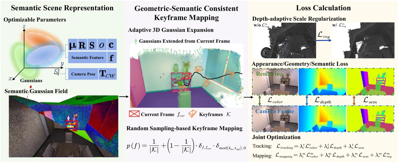
Figure 4. Overview of SG-Field, decoupled tracking, adaptive expansion, scale regularization, and random keyframe mapping.
Figure 5 explains forgetting as a shared-parameter effect. Suppose camera A first optimizes a set of Gaussians and camera B later observes an overlapping subset. B's update can overfit the shared primitives to its own viewpoint, reducing quality when A is rendered again. Random sampling does not remove parameter sharing. It instead prevents one local cluster from monopolizing the update budget and gives older views repeated opportunities to constrain the field.
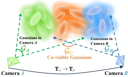
Figure 5. Shared Gaussians become overly fitted to later frames, degrading earlier views.
Figure 6 compares qualitative results on Replica and ScanNet. The synthetic scenes stress object outlines, texture, and highlights; the real scenes add imperfect labels and noisy depth. GS³LAM generally preserves sharper boundaries, but a qualitative plate is not a failure analysis. It does not show the distribution of errors by object distance, material, motion, or semantic class, all of which matter when the map is used by a robot.
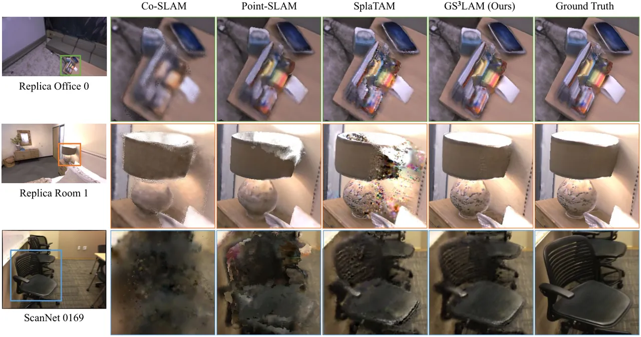
Figure 6. Qualitative rendering and semantic comparisons on Replica and ScanNet.
Interpretation and Open Questions
The strongest conceptual result is that semantic labels can act as a geometric regularizer. If a class boundary is consistently observed from many views, its feature error pushes the underlying ellipsoids to separate during rendering, not after reconstruction. This is different from semantic mapping as a post-process. The coupling also creates a new failure mode: inconsistent labels can pull the field toward contradictory surfaces, so label uncertainty deserves first-class treatment rather than being assumed away.
The paper does not establish long-term scaling. An explicit Gaussian field grows as the robot explores, and the reported mapping time is measured on one office scene. Memory, sorting cost, densification rate, and behavior after loop closure are not presented over long trajectories. A 4.29-second mapping step may be acceptable for an offline near-real-time reconstruction demo but is far from a conventional 30 Hz SLAM controller. Future evaluations should report memory peak and map size alongside accuracy.
Open-vocabulary perception is also outside the current scope. The decoder has a fixed output dimension and the system is trained with a predefined label set. A warehouse, hospital, or home deployment would need new categories, and incremental category learning may disturb old features. Combining SG-Field with language-aligned features is plausible, but the paper does not test whether such features remain stable under incremental updates or whether they preserve rendering speed.
Limitations
The authors explicitly acknowledge weaker average tracking than SplaTAM on Replica: 0.37 cm versus 0.36 cm ATE. This is not dismissed as noise. They explain that semantic detail and object edges are less useful for camera localization than prominent matching features. The result exposes a real multi-objective tension. Increasing semantic weight may improve boundaries while moving the pose optimum farther from the best tracking solution.
A second limitation is the behavior of explicit Gaussians under noisy depth. ScanNet contains depth errors that implicit NeRF systems can partly absorb through smooth MLP priors. A Gaussian field may instead encode the erroneous depth directly into primitive positions and scales. The paper suggests MLP-based attribute optimization as a possible remedy, and its average ScanNet ATE of 11.24 cm versus 0.37 cm on Replica shows how strongly domain and sensor quality affect the system.
A third limitation concerns evaluation completeness. The setup paragraph says five ScanNet subsets, while the tables report six scenes. Runtime is shown for only one Replica scene, semantic comparisons concentrate on Replica, and there is no dynamic-object, long-sequence, memory, or recovery study. These omissions do not invalidate the reported gains, but they limit how directly the result can be transferred to safety-relevant robot operation.
Conclusion
GS³LAM contributes more than a semantic channel attached to 3D Gaussian splatting. It defines a field in which appearance, geometry, and class features are updated together, then adds mechanisms for the specific ways incremental SLAM breaks: unknown pixels corrupt tracking, unexplored surfaces never enter the map, scales drift, and local keyframes overwrite older observations. The combination reaches 96.63% semantic mIoU on Replica, 36.26 dB average PSNR, and 109.12 FPS rendering while remaining competitive but not superior in tracking accuracy.
The next step should be to measure downstream utility rather than only map quality. A semantic SLAM system should be tested on navigation success, grasp selection, or human-robot query answering while reporting memory and failure recovery. Within the paper’s scope, the evidence supports a clear conclusion: shared multimodal Gaussian primitives can make dense semantic SLAM fast and accurate on controlled benchmarks. Outside that scope, label uncertainty, long-term scaling, and real sensor noise remain open engineering problems.
A semantic map becomes useful when every Gaussian is accountable for appearance, geometry, and class at the same time, and remains so after the camera moves on.