PAPER DEEP DIVE
GloSplat: Joint Pose-Appearance Optimization for Faster and More Accurate 3D Reconstruction
GloSplat unifies global structure from motion initialization with 3D Gaussian Splatting training through joint pose-appearance optimization. Its key design keeps explicit SfM feature tracks as independent optimizable geometry anchors instead of merging them with Gaussian means, so bundle adjustment can correct camera poses without being disrupted by densification or noisy photometric gradients. A retrieval-based variant prioritizes speed, while an exhaustive-matching variant targets maximum reconstruction quality; both improve the accuracy-speed frontier on unposed novel-view-synthesis benchmarks relevant to robot simulation reconstruction.
Authors: Tianyu Xiong, Rui Li, Linjie Li, and Jiaqi Yang
Paper: arXiv:2603.04847v1, March 5, 2026, cs.CV / cs.GR
Code availability: No public repository was found during this review. The paper says verification code is included in the supplementary material and the complete implementation will be released after acceptance.
Robotics relevance: The authors frame high-quality 3D reconstruction as infrastructure for robotic simulation. The experiments, however, evaluate novel-view-synthesis benchmarks only. They do not measure navigation, manipulation, simulator fidelity, latency inside a robot loop, or sim-to-real transfer.
Executive Summary
GloSplat changes the usual division of labor between structure from motion and 3D Gaussian Splatting. Instead of estimating camera poses once, freezing them, and then fitting Gaussians to the images, the system keeps camera poses trainable during splatting. It combines the image-space photometric objective with a reprojection objective computed from feature tracks. A separate set of sparse SfM landmarks remains available as geometric anchors, while the Gaussian means stay free to model appearance and local detail.
This design produces two variants. GloSplat-F uses retrieval-selected image pairs, XFeat, and LightGlue for fast reconstruction. GloSplat-A uses COLMAP-compatible SIFT features and exhaustive matching for higher quality. Across MipNeRF360, Tanks and Temples, and CO3Dv2, the fast version improves PSNR over VGGT-X by 1.37, 1.05, and 0.86 dB, respectively. At 1000 Courthouse images, it is reported to run 13.3 times faster than GPU-accelerated COLMAP. The high-quality version reaches 28.86 dB on MipNeRF360.
Why Pose and Appearance Need to Be Optimized Together
The standard Gaussian-splatting pipeline treats cameras as part of the input. SfM estimates intrinsics, extrinsics, and a sparse point cloud; the renderer then optimizes Gaussian position, covariance, opacity, and color against the training photographs. This works because the rendering loss is exceptionally good at fitting visible pixels. It also hides a strong assumption: every projected ray must be attached to the correct camera.
When that assumption fails, the renderer can compensate in ways that look plausible in training views and fail elsewhere. A Gaussian may move, stretch, multiply, or become nearly transparent in response to a pose error. The image loss can become small while the recovered scene geometry remains distorted. This is especially visible around thin structures: branches, leaves, wires, and object boundaries require several views to agree on the same spatial location.
Running a more elaborate SfM stage is one response, but it increases the preprocessing cost. Incremental SfM registers cameras one by one and repeatedly refines the reconstruction. Exhaustive matching grows rapidly as the number of images rises. A feed-forward pose predictor offers another route, but its accuracy may vary with scene scale, overlap, texture, and viewpoint distribution. The paper asks whether the reconstruction itself can supply enough geometric information to correct small or moderate pose errors without giving up the speed of a global initialization.
The difficulty is that photometric and geometric gradients do not optimize the same object. The photometric loss wants a rendered image to resemble its reference photograph. The feature-track loss wants the same sparse landmark to project near its observed pixel in every camera that sees it. If both gradients act directly on the same Gaussian position parameters, the renderer may move scene geometry to satisfy color while the sparse tracks drift through MCMC relocation. GloSplat therefore avoids a simplistic merge of camera, landmark, and Gaussian states.
The Main Design Choice
GloSplat keeps the SfM track landmarks, written as {Xk}, separate from Gaussian centers, written as {μj}. The cameras and track landmarks receive a bundle-adjustment signal from observed correspondences. The Gaussians receive the image-fitting signal. The correspondence graph links the two optimization processes without forcing them to share one parameter.
This is a subtle but important architectural decision. Sparse tracks are stable because they are tied to repeated feature observations, not to the current Gaussian density. They can therefore act as a geometric reference while Gaussians undergo densification, pruning, and relocation. The separation also limits a failure mode in which appearance gradients pull a Gaussian away from a well-supported landmark position and then the camera follows the displaced Gaussian, creating a self-consistent but incorrect solution.
System Architecture
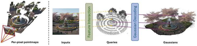
The pipeline contains three stages. The first stage builds local correspondences from unposed images. The second performs global SfM to initialize all cameras and sparse tracks. The third trains Gaussians while jointly refining camera poses with a feature-track bundle-adjustment term. The first two stages are frozen during Gaussian training, while the camera and Gaussian parameters remain active in the final stage.
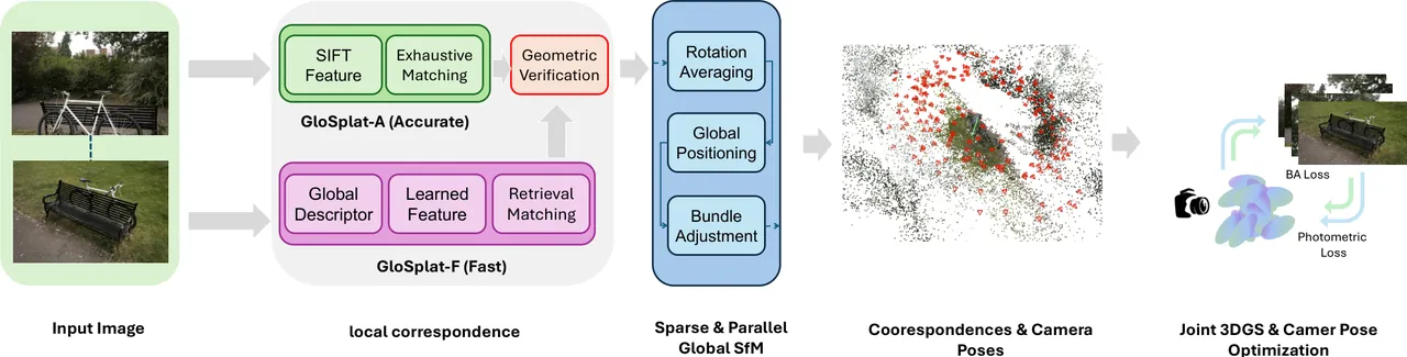
Figure 1: The paper's Figure 2 pipeline. Frozen correspondence extraction feeds global SfM; joint Gaussian and camera optimization then refines the reconstruction.
flowchart TD
  A["Unposed image set"] --> B["Frozen feature extraction"]
  B --> C{"Matching mode"}
  C -->|"Fast"| D["MegaLoc top-5
XFeat plus LightGlue"]
  C -->|"Accurate"| E["SIFT exhaustive matching"]
  D --> F["Global SfM"]
  E --> F
  F --> G["Global rotations
camera centers
SfM tracks"]
  G --> H["3DGS photometric training"]
  H --> I["Huber BA on track reprojection"]
  I --> J["Update cameras"]
  J --> H
  H --> K["Update Gaussian appearance"]
  K --> H
  I --> L["Keep track landmarks separate"]
  L --> I
The feedback loop is the substantive difference from a conventional pipeline. Photometric training improves the rendered scene, while reprojection training restrains camera motion relative to the observed tracks. The loop does not claim that all geometry is solved by one loss. It assigns each signal a different role and keeps the landmark state insulated from appearance-driven Gaussian operations.
Frozen Correspondence Preprocessing
GloSplat-F uses MegaLoc for image retrieval. Each image receives five candidate neighbors. XFeat extracts up to 4096 keypoints with 64-dimensional descriptors, and LightGlue predicts matches between selected pairs. The limited graph keeps matching cost from growing quadratically with the full image set. The fast route is optimized for scale, not for the maximum number of possible correspondences.
GloSplat-A uses SIFT features and exhaustive matching in a COLMAP-compatible setup. This creates a much denser verification graph and supplies more potential constraints for SfM and later bundle adjustment. The cost is evident in the runtime results, but the quality result shows that the joint optimizer can exploit the stronger tracks.
Both variants freeze feature extraction, matching, and pair retrieval. No reconstruction gradient flows back into the feature network or changes the selected edges. This keeps the correspondence graph stable across the 30000 Gaussian-training iterations. It also means that the method cannot repair a retrieval miss or a consistently incorrect descriptor match by learning a better representation. The authors identify this as an open limitation rather than claiming a fully end-to-end system.
Global SfM Initialization
The global SfM stage begins with rotation averaging. For a pair of cameras with a measured relative rotation, the system compares that measurement with the relative rotation implied by the global estimates. The robust objective is:
$$\mathcal L_{rot}=\sum_{(i,j)\in\mathcal E}\rho_{GM}\left(\left\|\log(R_{ij}^\top R_jR_i^\top)\right\|^2;\sigma\right)$$Here, E is the set of image pairs with relative observations, Rij is the observed rotation from camera i to camera j, and Ri and Rj are global camera rotations. The logarithmic map converts the residual rotation into a vector, while the robust kernel reduces the influence of erroneous pair estimates.
After global orientations are available, camera centers and landmarks must be positioned consistently. GloSplat uses the directional evidence from tracks. For landmark Xk, an observation in camera i imposes that the landmark should lie along the viewing ray represented by bip. The positioning objective is:
$$\mathcal L_{pos}=\sum_k\sum_{(i,p)\in\mathcal T_k}\left\|(I-b_{ip}b_{ip}^\top)(X_k-c_i)\right\|^2$$In this expression, ci is the center of camera i, Tk is the set of observations of track k, and I-bipbipT removes the component parallel to the viewing ray. The residual therefore measures lateral displacement from the ray rather than penalizing legitimate depth variation.
The initial pose and structure estimates are then refined with a Huber reprojection objective:
$$\mathcal L_{BA}^{SfM}=\sum_k\sum_{(i,p)\in\mathcal T_k}\rho_{Huber}\left(\|\pi_i(X_k)-x_{i,p}\|^2\right)$$The projection function πi maps a 3D track into camera i, and xi,p is its observed 2D feature position. Huber loss prevents a few mismatches from dominating the global solve. This stage is important because the later Gaussian optimizer needs a coherent starting reconstruction. It is not intended to freeze the final camera estimate forever.
Joint 3DGS and Bundle Adjustment
Once cameras and sparse tracks have been initialized, GloSplat trains Gaussian primitives with the standard image synthesis objective. The photometric loss combines an L1 term with structural similarity:
$$\mathcal L_{photo}=(1-\lambda_{SSIM})\|\hat I-I\|_1+\lambda_{SSIM}(1-SSIM(\hat I,I))$$The paper uses λSSIM=0.2. L1 provides a direct pixel-level error, while SSIM captures image structure that may be poorly represented by per-pixel differences. This objective can make a scene visually convincing across the training cameras, but it does not guarantee that a sparse landmark remains attached to the same physical point when the cameras move.
To preserve multi-view consistency, the system adds a Huber bundle-adjustment loss over the same SfM tracks:
$$\mathcal L_{BA}^{joint}=\sum_k\sum_{(i,p)\in\mathcal T_k}\rho_{Huber}\left(\|\pi_i(X_k)-x_{i,p}\|^2;\delta\right)$$The Huber threshold is fixed at δ=1.0. The residual is small when the current camera projects a track close to its detection and grows once the error exceeds the robust region. The complete training objective is:
$$\mathcal L=\mathcal L_{photo}+10^{-4}\mathcal L_{BA}^{joint}$$The BA weight is deliberately low. Photometric supervision covers many more measurements per image than the sparse correspondence set, so giving both terms equal weight would distort the appearance optimization. A coefficient of 10-4 lets the small geometric term steer the camera over many updates without overwhelming Gaussian fitting.
Camera pose parameters use Adam with a learning rate of 0.00001. The training schedule runs for 30000 iterations and permits at most 3 million Gaussians. The implementation uses the ngspalt rasterizer and a GPU cuDSS sparse solver for the joint problem. The reported overhead relative to ordinary training is about 3%, measured as roughly 31 minutes to 32 minutes in the paper's setup.
Why the Sparse Landmarks Are Not Gaussian Means
A natural shortcut would be to replace each SfM landmark with a Gaussian mean and run one reprojection loss on the Gaussian set. That removes duplicate geometry and makes the parameter graph simpler. It also couples the geometric residual to a state that MCMC densification may relocate at any moment. A Gaussian can be moved to improve color matching, split into smaller primitives, or be removed when it becomes redundant. Using such a moving state as the stable endpoint of a camera constraint is risky.
GloSplat instead lets the sparse tracks follow their own optimization path. The Gaussians can add detail and texture, while the track points retain a history of repeated observations. The ablation confirms that this is not a purely theoretical concern. Merging the two representations reduces GloSplat-A by 0.22 dB and GloSplat-F by 0.19 dB. The effect is consistent even though the two variants use different features and matching graphs.
The magnitude is not enormous, so the result should not be framed as evidence that one optimizer is the only workable design. It is better understood as a favorable bias in optimization dynamics. Separate anchors make pose updates less sensitive to local appearance rearrangements. That robustness matters most when geometry is thin, training views are unevenly distributed, or densification is aggressive.
Experimental Protocol
The evaluation uses MipNeRF360, Tanks and Temples, and CO3Dv2. MipNeRF360 combines object-centric and outdoor scenes with demanding view-dependent effects. Tanks and Temples stresses larger captures, with the paper reporting scenes of up to 1106 images. CO3Dv2 provides object-level multi-view data. PSNR and SSIM measure fidelity, while LPIPS captures perceptual differences. All runtime experiments use one NVIDIA RTX PRO 6000 with 96 GB of memory, a Ryzen 9 9950X CPU, and Ubuntu 24.04.
The fast route is compared with COLMAP-free methods, and the accurate route is compared with methods that use COLMAP poses. This distinction is essential when reading the tables. A number with a dagger in the paper denotes a result built on COLMAP poses. Comparing GloSplat-F only with the strongest COLMAP-initialized result can miss the intended tradeoff, while comparing GloSplat-A only with feed-forward systems can hide the cost of exhaustive matching.
| Method | MipNeRF360 | Tanks and Temples | CO3Dv2 |
|---|---|---|---|
| 3DGS† | 27.39 / .815 / .185 | 24.85 / .851 / .155 | 32.58 / .938 / .095 |
| MCMC† | 27.91 / .836 / .154 | 25.76 / .867 / .139 | 33.21 / .941 / .097 |
| MCMC | 22.19 / .548 / .282 | 21.42 / .679 / .278 | 25.71 / .712 / .201 |
| VGGT-X | 26.40 / .782 / .177 | 24.77 / .842 / .168 | 31.85 / .911 / .113 |
| GloSplat-F | 27.77 / .818 / .164 | 25.82 / .869 / .151 | 32.71 / .936 / .088 |
GloSplat-F improves over VGGT-X on every dataset in the table. The largest PSNR gain, 1.37 dB, appears on MipNeRF360. The Tanks and Temples gain is 1.05 dB, and the CO3Dv2 gain is 0.86 dB. The LPIPS improvement on CO3Dv2 is also substantial, from 0.113 to 0.088. These results matter because GloSplat-F does not use exhaustive matching, yet it can exceed a strong feed-forward pose-and-reconstruction baseline.
The fast method also reaches a useful region relative to COLMAP-initialized baselines. On MipNeRF360 it retains 99.5% of the PSNR of MCMC with COLMAP poses. On Tanks and Temples it slightly improves SSIM, with 0.869 versus 0.867, while keeping PSNR comparable. On CO3Dv2 it exceeds the COLMAP-initialized 3DGS result in both PSNR and LPIPS. The authors use these comparisons to argue that global initialization plus joint refinement can recover much of the quality previously associated with expensive pose preprocessing.
COLMAP-Compatible Accuracy
The exhaustive-matching route targets the quality ceiling instead of the fastest possible runtime. On MipNeRF360, GloSplat-A reaches 28.86 dB PSNR, .862 SSIM, and .139 LPIPS. Improved-GS is the closest strong baseline at 28.19 dB, .836, and .186. The PSNR improvement is 0.67 dB, SSIM rises by 2.6 points, and LPIPS is 25.3% lower.
| Method | PSNR ↑ | SSIM ↑ | LPIPS ↓ |
|---|---|---|---|
| 3DGS | 27.48 | .815 | .216 |
| AbsGS | 27.52 | .820 | .198 |
| PixelGS | 27.62 | .824 | .189 |
| MiniSplatting-D | 27.57 | .832 | .176 |
| TamingGS | 27.96 | .822 | .207 |
| 3DGS-MCMC | 28.01 | .835 | .186 |
| SteepGS | 27.05 | .795 | .247 |
| Perceptual-GS | 27.77 | .829 | .187 |
| Improved-GS | 28.19 | .836 | .186 |
| GloSplat-A | 28.86 | .862 | .139 |
The average metrics are not the whole story. The paper also reports per-scene results in its appendix. Strong object-centric CO3Dv2 scenes such as Apple, Skateboard, and Teddybear exceed 33 dB, while larger outdoor MipNeRF360 scenes remain harder. This variation is consistent with the method's dependence on correspondence coverage and global initialization quality. A high average does not mean every camera graph is equally favorable.
What the Ablations Reveal
The frozen-pose ablation is the clearest evidence that pose refinement is not decorative. With camera poses held fixed, PSNR falls to 19.18 dB, 8.59 dB below the full method. A photometric-only variant reaches 26.96 dB, 0.81 dB below the full result. The first comparison shows that a poor or unrefined camera estimate can severely damage reconstruction. The second shows that image reconstruction alone does not provide enough geometric stabilization.
Removing MCMC densification reduces PSNR to 26.02 dB, 1.75 dB below the full method. This suggests that camera correction and Gaussian capacity are complementary. A more accurate camera cannot represent branches or foliage if the primitive set is too limited, while a larger Gaussian set cannot resolve inconsistent observations if the camera trajectory remains wrong.
COLMAP exhaustive matching followed by joint optimization reaches 28.52 dB. The authors decompose the improvement into a 0.61 dB contribution from joint optimization and a 0.34 dB contribution from global SfM, corresponding to 64% and 36% of the reported gap. A COLMAP retrieval configuration without joint optimization drops to 17.93 dB, showing that a sparse retrieval graph is especially fragile when pose errors are left uncorrected.
Changing the local matcher produces a wide range. SuperPoint plus SuperGlue reaches 27.06 dB, 0.71 dB below the full GloSplat-F result. DISK falls to 19.65 dB, R2D2 to 17.54 dB, NetVLAD to 26.35 dB, and OpenIBL to 20.68 dB. DIR fails in the reported setting. These numbers temper the claim that joint optimization can compensate for arbitrary correspondence errors. It can refine useful tracks; it cannot invent missing views or stable matches.
Runtime and Scaling
The Courthouse experiment varies the input from 250 to 1000 images. At 250 images, GPU COLMAP takes 644.6 seconds, GloSplat-A 222.2 seconds, VGGT-X 53.9 seconds, and GloSplat-F 100.2 seconds. At 500 images, the times are 1165.0, 408.2, 113.3, and 191.9 seconds. VGGT-X is clearly the faster choice at small scale.
The ordering changes as the image set grows. At 750 images, VGGT-X takes 249.6 seconds and GloSplat-F takes 250.0 seconds. At 1000 images, GloSplat-F takes 327.8 seconds versus 398.9 for VGGT-X, 1371.3 for GloSplat-A, and 4349.2 for COLMAP. GloSplat-F therefore reaches a 13.3-times speedup over COLMAP and is about 1.2 times faster than VGGT-X. GloSplat-A is still 3.2 times faster than COLMAP while producing the highest-quality average in the main comparison.
| Input images | COLMAP | GloSplat-A | VGGT-X | GloSplat-F |
|---|---|---|---|---|
| 250 | 644.6 | 222.2 | 53.9 | 100.2 |
| 500 | 1165.0 | 408.2 | 113.3 | 191.9 |
| 750 | 2226.3 | 855.7 | 249.6 | 250.0 |
| 1000 | 4349.2 | 1371.3 | 398.9 | 327.8 |
The runtime result is a scaling argument rather than a universal speed guarantee. The fast route limits each image to a fixed number of retrieval neighbors, which prevents the matching graph from becoming fully dense. Global SfM estimates cameras in a parallel formulation instead of repeatedly registering one camera at a time. The benefit becomes visible when the number of images is large enough to amortize preprocessing and fixed setup costs.
The ScanNet comparison adds pose-error evidence. On scene 0301_00, COLMAP reports 133.83 degrees rotation error, 0.169 meters ATE, and 23.63 dB. 3RGS reports 9.30 degrees, 0.009 meters, and 30.11 dB. GloSplat-F reaches 7.82 degrees, 0.007 meters, and 31.24 dB. The other two reported scenes follow the same direction. This supports the claim that the joint term changes camera estimates, although the evaluation remains offline and should not be read as a real-time robot localization result.
| Scene | COLMAP R / ATE / PSNR | 3RGS R / ATE / PSNR | GloSplat-F R / ATE / PSNR |
|---|---|---|---|
| 0079_00 | 3.55 / .014 / 30.78 | 2.45 / .014 / 32.58 | 2.12 / .011 / 33.42 |
| 0301_00 | 133.83 / .169 / 23.63 | 9.30 / .009 / 30.11 | 7.82 / .007 / 31.24 |
| 0418_00 | 5.03 / .012 / 29.03 | 4.34 / .012 / 31.62 | 3.78 / .010 / 32.35 |
Qualitative Comparison
The Bonsai scene is a close-range object reconstruction with many small branches and leaves. It is a useful stress case because high-frequency detail must stay aligned across views. The paper reports 36.39 dB and 0.060 LPIPS for GloSplat-A, compared with 27.82 dB and 0.083 LPIPS for VGGT-X. The 8.57 dB PSNR difference is the strongest qualitative example highlighted by the authors.
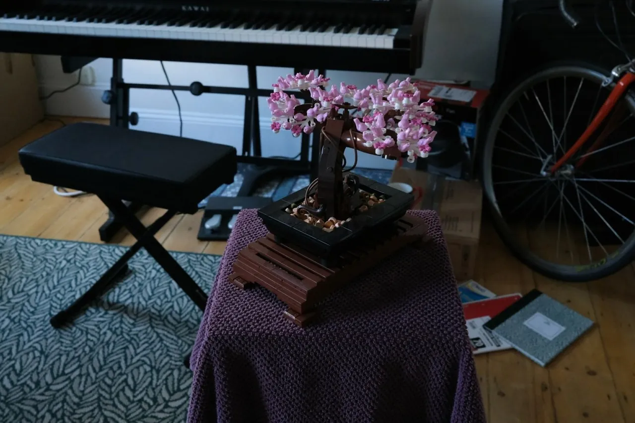
Figure 2: Ground-truth Bonsai view, corresponding to the first panel of the paper's Figure 4.
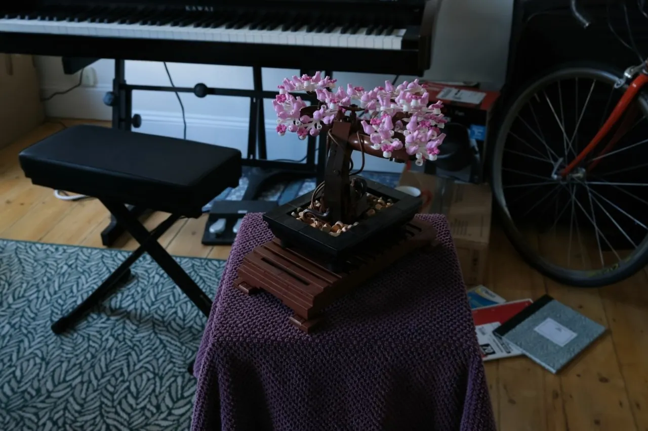
Figure 3: GloSplat-A on Bonsai, reported at 36.39 dB PSNR and 0.060 LPIPS.
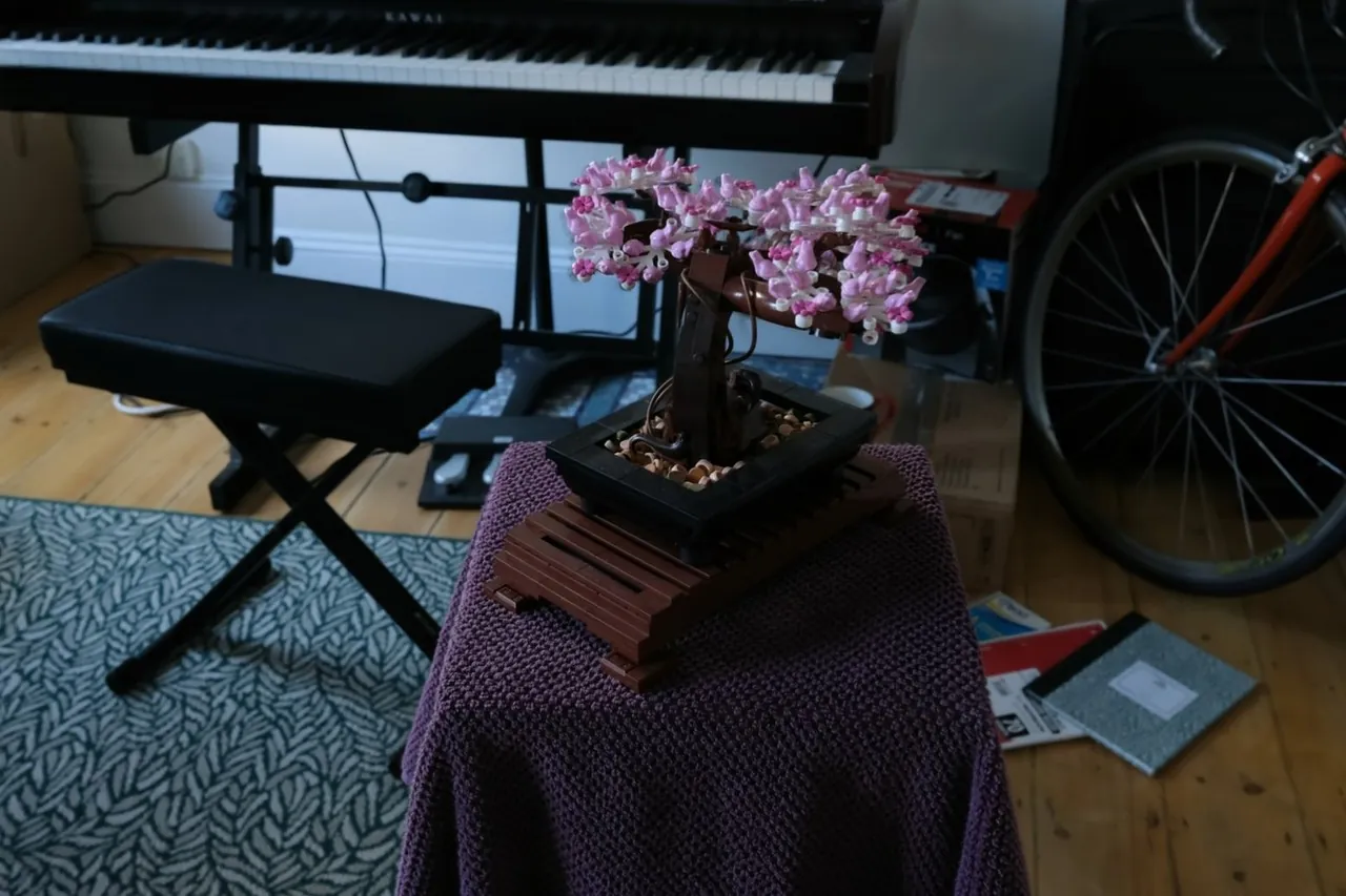
Figure 4: GloSplat-F on Bonsai. This is the retrieval-based, lower-cost reconstruction path.
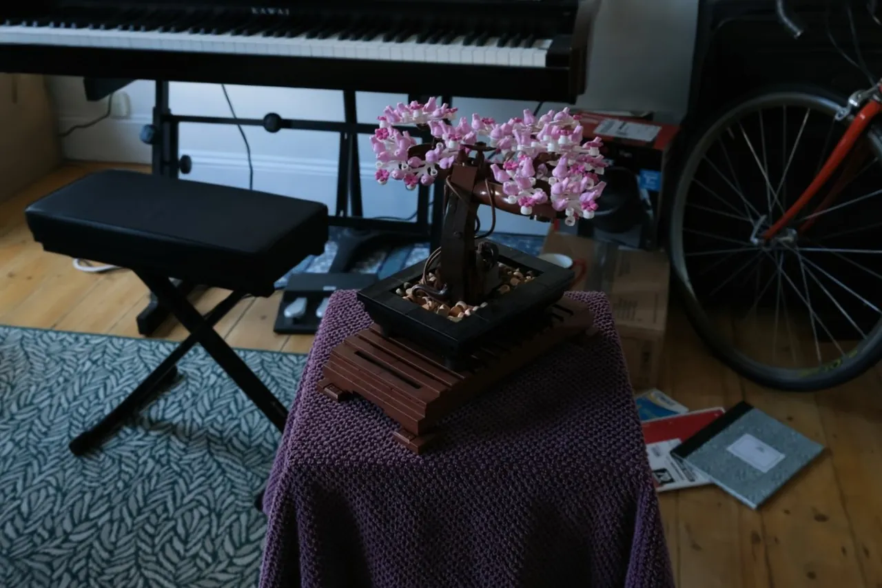
Figure 5: VGGT-X on Bonsai, reported at 27.82 dB PSNR and 0.083 LPIPS.
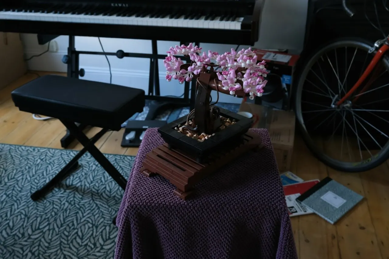
Figure 6: Improved-GS on Bonsai, one of the strong COLMAP-based reconstruction baselines.
The Flowers example focuses on fine petals and dense vegetation. GloSplat-A reports 24.88 dB and 0.147 LPIPS, while VGGT-X reports 18.13 dB and 0.273 LPIPS. That is a 6.76 dB PSNR gain and an approximately 46% LPIPS reduction. The failure mode in this kind of scene is not simply a lack of texture. Small pose errors can blur the silhouette of a petal or split a thin stem into several inconsistent surfaces.
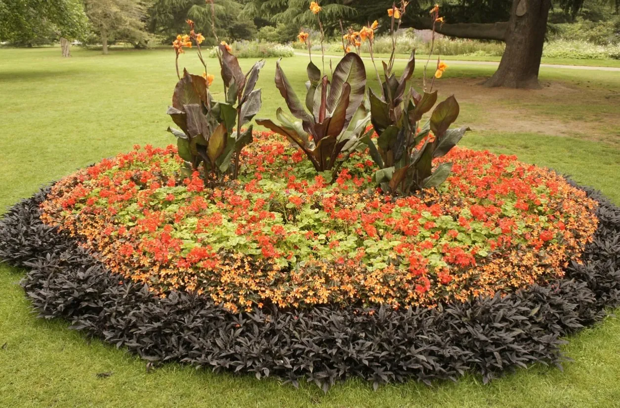
Figure 7: Ground-truth Flowers view with dense petals and fine leaves.
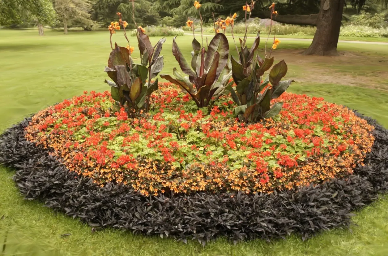
Figure 8: GloSplat-A on Flowers, reported at 24.88 dB PSNR and 0.147 LPIPS.
The paper also includes Garden, where it reports a 5.69 dB gain over VGGT-X. Across the three examples, the claimed improvement is concentrated around complex structure and fine edges. Yet the paper does not include a user study, a systematic crop comparison, or a dedicated failure gallery. The qualitative panels therefore support the mechanism but cannot establish perceptual superiority for every scene category.
Limitations and Open Questions
The first limitation is explicitly acknowledged by the authors: correspondence preprocessing remains frozen. Gradients do not flow through feature extraction, matching, or retrieval. If top-five retrieval misses informative views, the global SfM stage can inherit a weak graph, and the joint optimizer cannot recover observations that were never supplied. The method improves pose refinement within the correspondence graph; it does not solve view selection or feature learning jointly.
The second limitation is the scope of the evaluation. The paper motivates reconstruction as a component of robot simulation, but all quantitative experiments measure novel-view synthesis or pose error on familiar static datasets. There is no robot navigation, manipulation, collision checking, physics simulation, or sim-to-real task. There is also no measurement of long sequential robot video with motion blur, rolling shutter, dynamic objects, or temporary loss of tracking.
The third limitation is resource behavior. The maximum of 3 million Gaussians and 30000 training iterations imply substantial memory and compute requirements. The reported 3% overhead is useful because it isolates the cost of joint optimization relative to training, but it is not a complete deployment budget. The paper does not provide peak memory, end-to-end energy, failure rates on very large scenes, or recovery behavior after a bad initialization.
A fourth issue is experimental attribution between GloSplat-F and GloSplat-A. The variants differ in feature type, matching strategy, and graph density at the same time. Their reported quality gap therefore cannot be interpreted as a one-variable ablation. A robotics team choosing between them should benchmark on its own camera trajectory, image count, view overlap, and latency target rather than using a single Courthouse scaling curve.
There is also an important distinction between a stable landmark and a correct landmark. Separation protects a track from Gaussian relocation, but it cannot repair a systematically biased track. If an object has repetitive texture, if a moving object contributes false matches, or if the retrieval graph links visually similar but physically different views, the BA term can consistently constrain the camera toward the wrong geometry. Robust Huber loss reduces the influence of outliers, but it is not a semantic consistency mechanism.
For RobotWorld readers, GloSplat is most credible as a reconstruction architecture, not yet as a demonstrated robotics system. The dense robot loop would need a different validation suite: repeated traversals, low-overlap sequences, calibration drift, real-time keyframe selection, and reconstruction quality measured by downstream task success. Those tests would reveal whether the method's nominal speed and geometric gains survive the acquisition conditions that matter outside benchmark archives.
Engineering Takeaways
The paper offers a clean separation of concerns. Track landmarks answer where a repeated observation should project. Gaussians answer what the scene should look like. Cameras sit between them and receive a deliberately weak geometric correction so that the appearance optimizer cannot freely redefine the coordinate system. This division is more transferable than any one implementation detail.
The scale result also suggests a practical design rule. If a robot platform can afford a fixed-size retrieval graph and a global initialization pass, a fast joint reconstruction route may beat a fully feed-forward pipeline once the capture contains enough images. For smaller clips, the feed-forward model may remain the better latency choice. The crossover is workload dependent, and the paper's 750 to 1000 image behavior is a useful starting point for that decision.
The most important missing engineering step is uncertainty. A production robot needs to know when pose refinement is trustworthy. The current method reports aggregate pose errors, but it does not expose a per-camera confidence that could trigger re-observation, keyframe replacement, or a fallback to frozen poses. Pairing the sparse geometric residual with a calibrated uncertainty estimate would make the idea more useful for manipulation and navigation, where a silent pose drift can be more damaging than a visible rendering defect.
Conclusion
GloSplat treats camera poses as variables during Gaussian-splatting training, but it does so with a carefully bounded geometric signal. Global SfM supplies a coherent initialization and sparse feature tracks. The photometric loss improves appearance. A low-weight Huber reprojection loss continuously corrects camera estimates, while a separate set of track landmarks prevents MCMC relocation from rewriting the geometric anchor.
The evidence is strong within its stated scope. The fast variant beats VGGT-X on three NVS benchmarks, scales better at large image counts, and approaches COLMAP-initialized quality. The accurate variant reaches 28.86 dB on MipNeRF360 and improves pose metrics on ScanNet. The main scientific question left open is whether these gains remain dependable in continuous robot data, under severe overlap loss, and with real latency and memory constraints.
Golden Quote
The camera may learn from appearance, but appearance should not be allowed to redefine the geometric anchor. GloSplat keeps one stable track reference beside every Gaussian experiment.
SOURCE LINKS