Safe Interval Motion Planning for Quadrotors in Dynamic Environments

Paper: Safe Interval Motion Planning for Quadrotors in Dynamic Environments
Authors: Songhao Huang, Yuwei Wu, Yuezhan Tao, and Vijay Kumar
Venue: IEEE ICRA 2025, pp. 2780-2786
Full text: arXiv:2409.10647 | DOI: 10.1109/ICRA55743.2025.11127946
Implementation: KumarRobotics/SIMP, reviewed at commit 401262c

Executive summary: The paper couples edge-level safe intervals with a dynamic visibility graph, separates candidate routes by temporal topology, and optimizes a B-spline inside connected 4-D corridors. The result is a planner that remains safe and dynamically executable while producing substantially smoother trajectories in moving-obstacle fields.

Problem Setting and Motivation

Most high-quality quadrotor planners begin from a static occupancy map. That abstraction is useful, but it fails when a person, vehicle, or another robot crosses the intended route during execution. Frequent replanning against successively updated maps can react to the current state, yet it does not explicitly reason about when a narrow passage will be available in the near future.

A natural alternative is to add time as a fourth state dimension. The resulting search can represent waits and moving gaps, but the state space expands rapidly. Most four-dimensional samples in a bounded time horizon correspond to combinations that never conflict, and exhaustive search becomes difficult to run within a flight controller's planning budget.

Safe-interval planners reduce this burden by replacing individual time steps with maximal intervals during which a state or edge remains safe. Grid-based safe-interval search has a strong foundation, but applying it directly to dense 3-D maps can create expensive per-cell temporal preprocessing. The paper therefore asks how safe intervals can be retained without paying the full cost of a temporal grid.

Probabilistic roadmaps provide the complementary spatial tool. They express long visibility connections with relatively few vertices and naturally produce multiple routes. However, a conventional roadmap evaluates geometry. In a dynamic scene, two routes can share the same geometric shape while crossing the same opening at different times, leading to different collision outcomes.

The proposed architecture combines these ideas at the level of graph edges. Every visible connection carries its own time windows, adjacent edges must agree on compatible timing, and candidates are classified not only by spatial shape but also by temporal deformation. The back end then treats each selected route as the seed for a spatial-temporal corridor and performs trajectory optimization inside that corridor.

Definitions That Carry the Method

The environment is assumed to be fully observed over a finite horizon, and moving-obstacle trajectories are known with bounded dynamics. At any time, space is divided into free and occupied regions:

$$\mathbb{R}^{3}=\mathcal{X}_{\mathrm{free}}^{t}\cup\mathcal{X}_{\mathrm{obs}}^{t},\qquad \forall t\in[t_s,t_e].$$

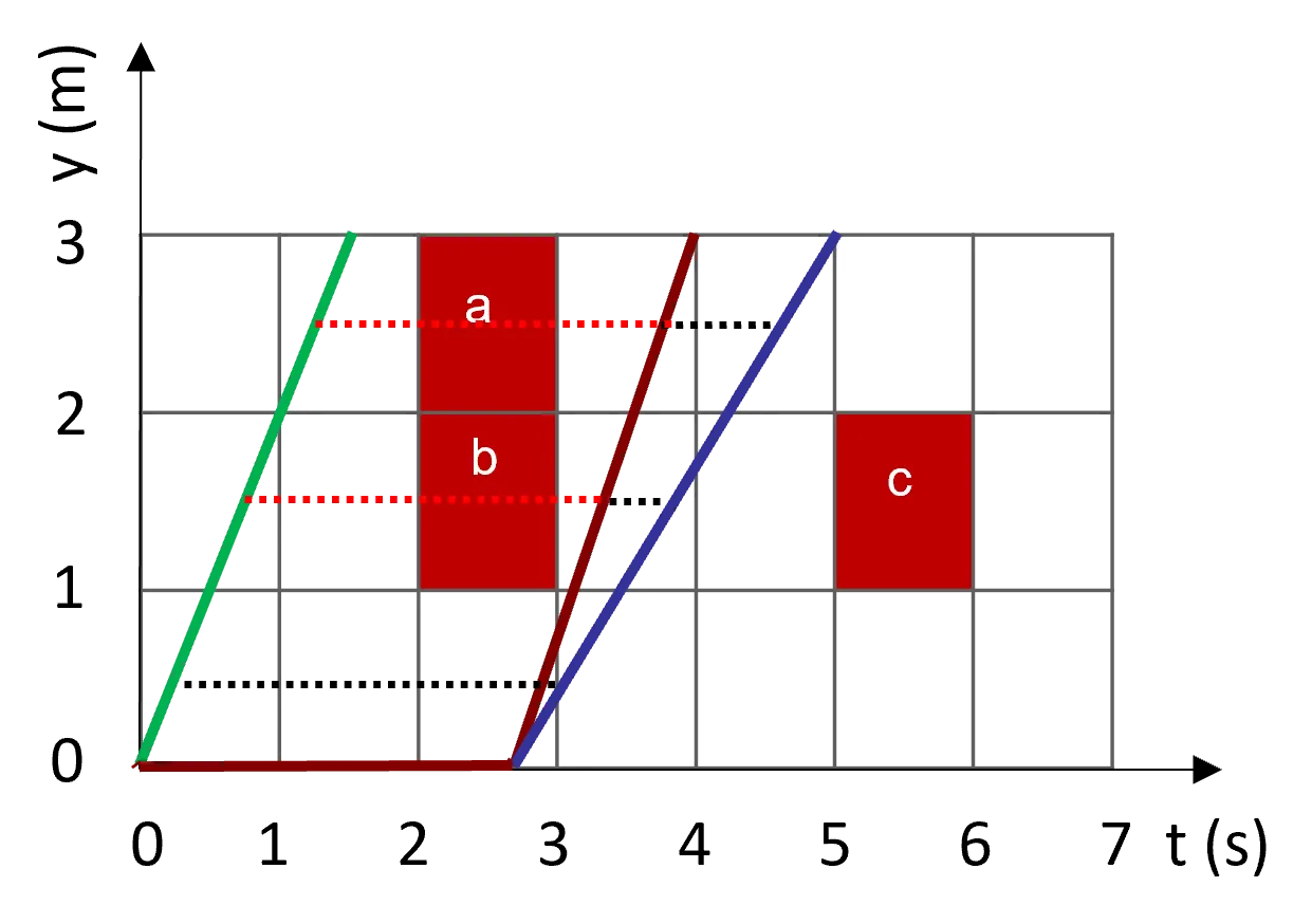
For an edge $e$, let $\mathrm{CI}(e)$ denote the union of times at which the edge intersects a moving obstacle. The safe intervals are the portions of the remaining time that are long enough for the vehicle to traverse the edge:

$$(t_j,t_{j+1})\in T\setminus\mathrm{CI}(e),\qquad t_{j+1}-t_j>t_{\min}.$$

The duration filter is central rather than cosmetic. A geometric gap that disappears before the quadrotor can physically cross it is not a useful connection. The paper estimates $t_{\min}$ with a trapezoidal velocity profile under zero start and end velocity, thereby embedding a lower-order dynamic criterion in the graph before nonlinear trajectory optimization begins.

Safety must also propagate through connected edges. A path is temporally realizable when the safe intervals of every consecutive pair overlap at their shared vertex. The resulting sequence of intervals forms a directed temporal corridor. Later optimization can alter the exact timing, but it cannot escape the connected safe windows without paying the corridor penalty.

Topological diversity is handled through Uniform Temporal Visibility Deformation (UTVD). Given two parameterized trajectories, UTVD allows a positive affine reparameterization in time and checks whether corresponding points can be joined by collision-free visibility segments:

$$s'=\alpha s+\theta,\qquad \sigma_1(0)=\sigma_2(\theta),\qquad \sigma_1(1)=\sigma_2(\alpha+\theta).$$

Here $\alpha$ controls time scaling and $\theta$ controls temporal shift. Endpoint matching aligns the comparison, while collision checking is performed over the corresponding time range of each segment. This avoids two common errors in dynamic topology evaluation: comparing paths that do not start or end at the same instant, and collapsing distinct avoidance decisions into one class merely because their spatial routes look similar.

Front End: A Visibility Graph with Timed Edges

The spatial map is represented as a 3-D occupancy grid. Each moving obstacle is represented by a bounded ellipsoid whose center follows a polynomial trajectory. For every candidate graph edge, the implementation creates a cuboid around the line and inflates it by the Minkowski sum of the quadrotor and obstacle geometry. Intersections between the obstacle trajectory and the cuboid boundaries determine collision times.

Edge-level safety is stricter than vertex-only checking. Two endpoints can both be safe while the straight connection passes through a moving object. Checking the entire edge removes this failure mode and permits longer visibility connections, which is important for reducing graph density.

The graph contains Guards and Connectors. The start and goal are Guards. A sample that sees exactly two Guards may become a Connector if its incident edge intervals overlap; a sample without such a connection becomes a new Guard. Heuristic sampling favors regions with few Connectors, and a finite sample budget controls graph construction.

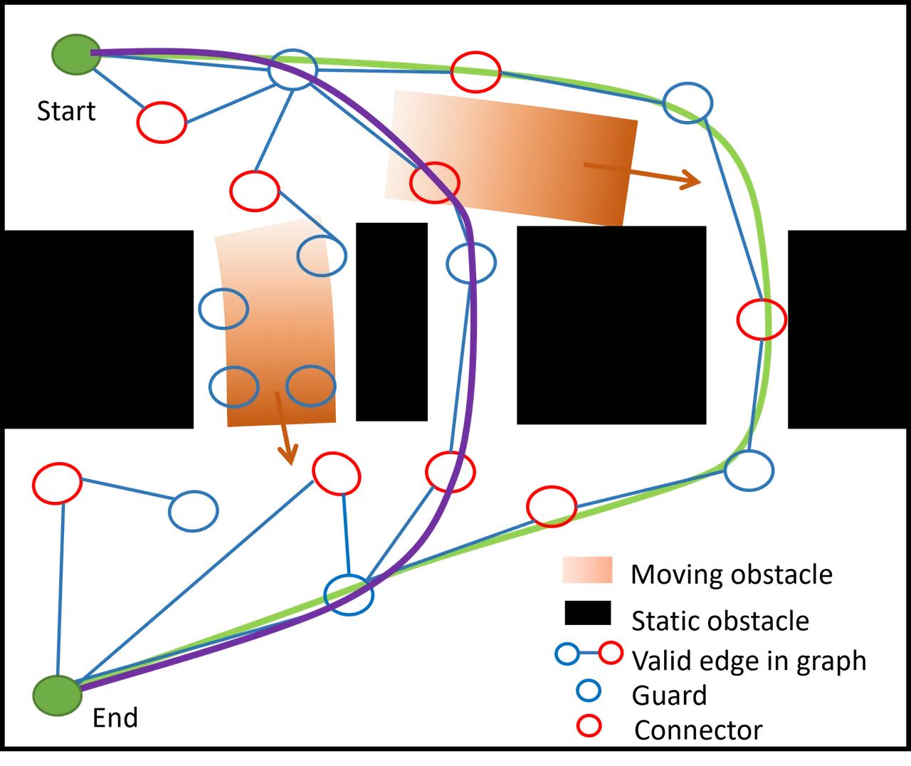
When a candidate connection is compared with a neighboring route, time-stamped samples are used for the UTVD test. If the new route is equivalent and shorter, it can replace the old vertex. If it is topologically distinct, it is retained. This is the mechanism that prevents the graph from representing only the first geometric detour found by the sampler.

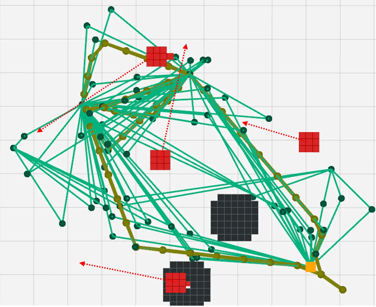
Depth-first search then extracts multiple distinct paths. Vertex timing follows an earliest-arrival rule before the initial temporal corridor is passed to the optimizer. Figure 3(b) illustrates a front-end result with static obstacles, moving objects, a dense green visibility graph, and several yellow candidate routes.

The released code makes the four-dimensional state explicit: graph nodes store position, time, and interval data, while line queries are cached by geometry and time range. The following excerpt is the concrete implementation of edge safe-interval lookup:

// src/kr_dyn_planner/plan_core/include/path_searching/dyn_topo_prm.hpp:572
inline bool DynTopoPRM::findSafeIntervalsForLineCached(
    const Eigen::Vector3d& pt1, const Eigen::Vector3d& pt2,
    const Eigen::Vector2d& time_range,
    std::vector<Eigen::Vector2d>& intervals) const
{
    const LineQueryKey key = makeLineQueryKey(pt1, pt2, time_range);
    const auto cached = line_interval_cache_.find(key);
    if (cached != line_interval_cache_.end()) {
        intervals = cached->second.intervals;
        return cached->second.valid;
    }

    LineQueryValue value;
    value.valid = CollisionChecker_->findSafeIntervalForLine(
        pt1, pt2, time_range, value.intervals,
        speed_limit_, acc_limit_);
    line_interval_cache_.emplace(key, value);
    intervals = value.intervals;
    return value.valid;
}

The cache key includes a quantized time range in addition to both endpoints. This is consistent with the paper's semantics: a fixed line may be safe at one departure time and blocked at another. Caching only by spatial coordinates would turn a useful multi-query optimization into a source of incorrect path connections.

From Route to Safe Region

A graph path alone is too thin to support high-quality optimization. If the B-spline is kept near invisible edge centerlines, the smoother and dynamic-feasibility terms may have little room to operate. The paper therefore expands each route into coupled spatial and temporal corridors.

Successive seed points are selected along each edge. Around every seed, an axis-aligned cuboid is inflated in three dimensions. At each expansion step, the planner tests whether the cuboid remains collision-free during the relevant time interval. The output is not a static box with a time label attached afterward; it is a pair consisting of a spatial cuboid and the interval over which that cuboid is valid.

Connected paths require more than spatial adjacency. Consecutive corridor boxes must overlap in space and in time. This guards against a trajectory that moves continuously through the boxes but reaches a later box after its safe interval has ended. The released planner checks these two overlap conditions before handing a candidate to the nonlinear optimizer.

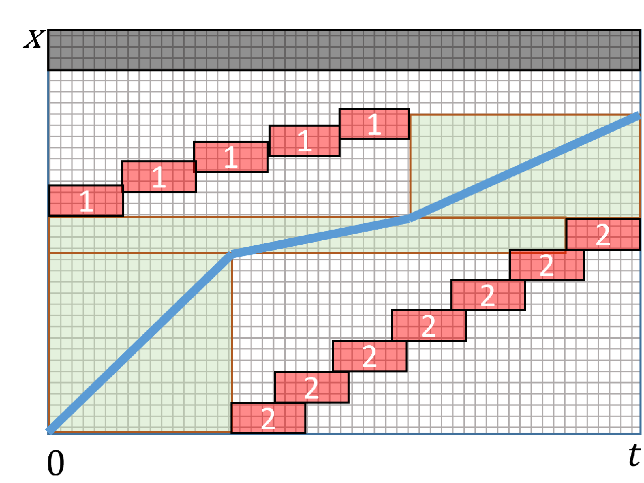
The axis-aligned representation is tractable but conservative. It simplifies collision queries and permits simple distance-to-box costs, although it may leave usable space unused in strongly rotated passages. For an online planner, that conservatism is a deliberate trade: repeated probabilistic sampling with a more general polytope could consume the budget needed for optimization.

Back End: B-Spline Optimization in Space and Time

Quadrotors are differentially flat, so a smooth trajectory can be represented through a small set of flat outputs. The method uses a uniform B-spline and optimizes its control points with a time allocation strategy. The convex-hull property links the continuous curve to constraints imposed on or near its control points.

The composite objective contains four terms:

$$\min_{\mathbf Q,\mathbf t}\sum_{d\in D}\lambda_d J_d(\mathbf Q,\mathbf t),\qquad D=\{c,od,ct,f\}.$$

Control effort, dynamic-obstacle clearance, spatial-temporal corridor membership, and dynamic feasibility are represented by $J_c$, $J_{od}$, $J_{ct}$, and $J_f$. The corresponding weights are $\lambda_d$. The optimizer updates control points and refines trajectory timing, then selects the candidate with the lowest control effort among the available topological paths.

Higher-order control points are obtained from finite differences of the primary control points:

$$\mathbf V_i=\frac{\mathbf Q_{i+1}-\mathbf Q_i}{t_s},\quad \mathbf A_i=\frac{\mathbf V_{i+1}-\mathbf V_i}{t_s},\quad \mathbf J_i=\frac{\mathbf A_{i+1}-\mathbf A_i}{t_s}.$$

Smoothness is imposed through a sum of squared jerk magnitudes:

$$J_c=\sum_{i=p_b-3}^{N_c-p_b}\|\mathbf J_i\|_2^2.$$

The dynamic-feasibility term penalizes velocity and acceleration values relative to their specified limits. The search stage uses a lower-order approximation; this term retains the higher-order differences that must ultimately be respected by the continuous spline:

$$J_f=\sum_{i=p_b-1}^{N_c-p_b}\|\mathbf V_i-v_m\|_2^2+\sum_{i=p_b-2}^{N_c-p_b}\|\mathbf A_i-a_m\|_2^2.$$

For corridor membership, a control point is associated with the cuboid whose temporal interval contains its knot. Let $b_{l,j}$ and $b_{u,j}$ be the lower and upper cuboid bounds. The violation is measured with an L1 distance:

$$J_{ct}=\sum_{i=p_b}^{N_c-p_b}\left(\|b_{l,j}-\mathbf Q_i\|_1+\|\mathbf Q_i-b_{u,j}\|_1\right).$$

Moving obstacles are modeled as ellipsoids rather than points. If $E_j$ is the coefficient matrix for obstacle $j$, then the normalized distance between trajectory point $p_i$ and obstacle center $o_j$ is:

$$d(p_i,o_j)=\left\|E_j^{-1}(p_i-o_j)\right\|_2.$$

The obstacle term applies a quadratic penalty only when this normalized distance falls below a threshold:

$$J_{od}=\sum_{i=0}^{m}\sum_{j=0}^{k}\left(\max\left(0,d(p_i,o_j)-d_{th}\right)\right)^2.$$

These terms have different jobs. The corridor cost defines the feasible region inherited from graph search. The obstacle cost prevents the continuous curve from grazing a moving ellipsoid inside that region. Smoothness and feasibility shape the resulting motion. Using any one term alone would leave an important failure mode uncovered.

flowchart TD
    A[Static occupancy and predicted obstacle paths] --> B[Form and inflate graph edges]
    B --> C[Solve edge collision intervals]
    C --> D[Discard intervals shorter than t_min]
    D --> E[Build Guards and Connectors]
    E --> F[Compare routes with UTVD]
    F --> G[Extract distinct topology classes]
    G --> H[Inflate cuboids and valid time intervals]
    H --> I[Reject disconnected space-time corridors]
    I --> J[Optimize B-spline control points]
    J --> K[Control effort, feasibility, obstacle, corridor]
    K --> L[Choose the lowest-control-cost candidate]

The public planner_manager code exposes the same separation. It requests topological paths, obtains their corridors and intervals, validates connectivity, and only then calls the back-end optimizer. The excerpt below captures that interface:

// src/kr_dyn_planner/plan_core/src/planner_manager.cpp:335
bspline_optimizer_rebound_->dyn_topo_prm_->findTopoPaths(
    local_start_pt, local_end_pt, world_start_time, duration,
    start_pts, start_ts, topo_graph, topo_paths);
if (topo_paths.empty()) {
    ROS_ERROR("No path found.");
    return false;
}

std::vector<std::vector<Eigen::Vector2d>> topo_sfc_intervals;
std::vector<std::vector<Eigen::Matrix<double, 3, 2>>> topo_sfc_cuboids;
bspline_optimizer_rebound_->dyn_topo_prm_->getSFC(
    topo_sfc_cuboids, topo_sfc_intervals);

for (size_t i = 0; i < candidate_count; ++i) {
    if (!validateConnectedSFC(topo_sfc_cuboids[i],
                              topo_sfc_intervals[i],
                              spatial_overlap_min,
                              time_overlap_min, &reason)) {
        continue;
    }
}

The optimizer implementation assembles smoothness, feasibility, dynamic-obstacle distance, and corridor costs into one weighted objective and gradient. The code comment is particularly relevant to reproducing the paper: corridor membership is checked on sampled points of the continuous spline, not only on control points, because a spline can leave a cuboid even when all control points appear acceptable.

Simulation Design

The authors evaluate three environment classes with increasing static and dynamic complexity. Occupancy density ranges from $[0,0.01]$ in the sparse case to $[0.05,0.1]$ in the moderate case and $[0.15,0.2]$ in the dense case. The corresponding ranges for moving obstacles are $[0,20]$, $[20,40]$, and $[40,60]$.

Each class contains 100 trials. The map is regenerated every three trials, which reduces correlation among nearby trials while retaining enough repetitions to estimate success rate. Start and goal positions are sampled in collision-free regions, and a trial succeeds when a collision-free path or trajectory reaches the goal.

Environment	Occupancy density	Moving obstacles	Trials	Map refresh
Sparse	[0, 0.01]	[0, 20]	100	Every 3 trials
Moderate	[0.05, 0.1]	[20, 40]	100	Every 3 trials
Dense	[0.15, 0.2]	[40, 60]	100	Every 3 trials

The front-end benchmark compares the method with T_PRM, VIS_PRM, SIPP, and SIPP_IP. Dynamic variants of the probabilistic planners replace constant-speed edge traversal with a trapezoidal velocity profile. The reported metrics are success rate, computation time, path length, and flight time.

The qualitative ordering is informative. Grid-based safe-interval methods pay for temporal preprocessing over many cells and degrade as the map becomes denser. T_PRM is fast and accurate enough to find routes, but limiting edge length to make vertex checks safe produces more convoluted paths. VIS_PRM loses success as the number of moving objects increases because its sampled temporal connections do not provide the same edge-level completeness.

The dynamic checks affect the baselines differently. T_PRM(dyn) loses success and gains flight time, showing that a maximum edge-length heuristic does not fully encode the ability to traverse an edge within a safe interval. VIS_PRM(dyn) changes less because randomly assigned vertex times often provide generous traversal durations. SIPP_IP is the slowest and frequently exhausts its expansion limit.

Trajectory Quality and Hardware Evidence

The trajectory comparison uses TPRMO, which combines a temporal PRM front end with moving-obstacle distance costs but no spatial-temporal corridor. The experiment runs 100 trials per map class and evaluates the trajectory after one optimization pass. Table I reports success, path length, flight time, and average control cost.

Environment	Method	Success	Path length	Flight time	Control cost
Sparse	Proposed	100%	7.66 m	6.04 s	17.71 m2/s5
Sparse	TPRMO	99%	7.89 m	5.55 s	72.67 m2/s5
Moderate	Proposed	98%	7.93 m	6.05 s	26.20 m2/s5
Moderate	TPRMO	97%	8.11 m	5.72 s	73.27 m2/s5
Dense	Proposed	97%	7.44 m	5.69 s	30.53 m2/s5
Dense	TPRMO	97%	7.52 m	5.36 s	70.31 m2/s5

The one-time success rates are close, with a two-point advantage in the sparse class and a one-point advantage in the moderate class. The decisive result is control effort. The proposed planner reduces average cost from 72.67 to 17.71 in sparse maps, from 73.27 to 26.20 in moderate maps, and from 70.31 to 30.53 in dense maps. These correspond to reductions of roughly 75.6%, 64.2%, and 56.6%.

The proposed trajectories are also 1.1% to 2.9% shorter, while their flight times are 5.8% to 8.8% longer. The longer duration is not a contradiction: the optimizer spends more time where necessary to achieve gentler changes in acceleration and a safer placement inside the corridor. In the dense environment, both methods reach 97% success, so the advantage is trajectory quality rather than an isolated success-rate gain.

Environment	Control-cost reduction	Path-length change	Flight-time change	Success-rate change
Sparse	About 75.6%	About 2.9% shorter	About 8.8% longer	99% to 100%
Moderate	About 64.2%	About 2.2% shorter	About 5.8% longer	97% to 98%
Dense	About 56.6%	About 1.1% shorter	About 6.2% longer	97% to 97%

The hardware setup uses two Scarab ground robots as moving obstacles. Each Scarab carries a $0.91\,\mathrm{m}\times0.16\,\mathrm{m}$ cylinder and follows a rectangular trajectory. Three static cylinders measure $1.2\,\mathrm{m}\times0.3\,\mathrm{m}$. The aerial platform is a customized Dragonfly 230 with a VOXL flight board, a forward time-of-flight camera, and a downward tracking camera. Vicon supplies a common reference frame and odometry.

In the demonstrated run, the quadrotor starts in the lower-right corner while the ground robots continue moving. It plans toward a goal above a black box, tracks the generated trajectory through the gaps, and receives subsequent goals after arrival. The upper-right inset in Figure 7 shows the spatial-temporal corridor and the selected low-control-cost path.

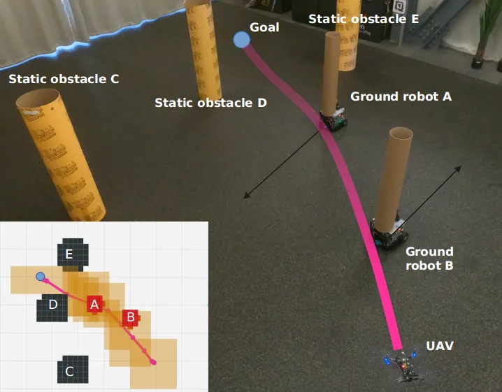
The top-down view in Figure 2 makes the timing of the decision clearer. Moving robots appear as red regions, static obstacles as black regions, and odometry directions as green arrows. The plan reflects the predicted ordering of occupied regions, rather than a purely instantaneous repulsive response.

Claimed Guarantees and Their Practical Meaning

The paper connects its argument to SIPP's completeness and resolution-optimality results. SIPP is complete and resolution-optimal for the stated grid representation when dynamic constraints and action availability are not the limiting factors. The proposed method introduces a PRM-style graph, edge safe intervals, and lower-order dynamic bounds, so its formal statement is probabilistic completeness and optimality within a finite duration under the assumption that the environment is representable by the graph.

This is a conditional guarantee, and the condition matters. If the sampler never creates the vertices needed for a valid passage, the graph cannot return that passage regardless of how strong the optimizer is. Increasing time and sample limits improves coverage, but online operation always imposes a cutoff. The method's practical reliability therefore depends on the relation among map geometry, sample radius, obstacle speed, and planning budget.

The trapezoidal profile supplies a useful lower bound on edge traversal time, but it does not solve the complete high-order trajectory problem in the front end. The B-spline optimizer is still necessary to enforce smoothness and dynamic feasibility. A corridor may be temporally valid under the lower-order model yet remain difficult to optimize if the corridor is narrow, the allocated interval is short, or the obstacle penalty conflicts with the corridor boundary.

Candidate selection also inherits the cost weights. The paper emphasizes the minimum-control-cost candidate, which is sensible for smoothness, but the resulting safety margin is influenced by the dynamic-obstacle threshold and corridor geometry. A deployment should validate margins against the actual state estimator, controller tracking error, rotor saturation, and obstacle prediction uncertainty rather than treating the simulated separation as a universal certificate.

Limitations

The authors explicitly identify onboard perception and more complex motion patterns as future work. Their current system relies on known obstacle trajectories or an external mapping pipeline, and the real-world obstacles follow relatively structured rectangular paths. This does not establish the same performance for occlusions, late detections, sudden direction changes, or human motion that violates the prediction model.

A second limitation is the dependence on graph representability. The probabilistic guarantee assumes adequate sampling coverage, and the graph construction has finite time and sample budgets. Narrow passages that require long visibility edges or a rare sequence of vertices may be missed. More samples improve coverage but consume the planning time needed for corridor construction and optimization.

A third limitation is deterministic prediction. A polynomial obstacle trajectory collapses uncertainty into a single future centerline. If the predicted path is shifted or the ellipsoid size is underestimated, the computed safe intervals may include a collision. Robust deployment would need to propagate state-estimation and prediction uncertainty into the interval boundaries and the nonlinear obstacle cost.

A fourth limitation is the scope of hardware evidence. The simulation study uses 100 trials per density class, while the hardware section presents a representative experiment rather than a large repeated trial set. The real platform demonstrates integration with motion capture, a flight controller, and moving ground robots, but it does not provide statistical estimates for hardware success across many scenes.

A fifth engineering limitation is the conservative cuboid representation. Axis-aligned corridor inflation is fast and compatible with gradient-based optimization, but rotated or curved free regions can be represented inefficiently. A more expressive corridor may improve feasible volume at the cost of more complex collision checks and constraints.

Conclusion

The paper's main contribution is not a single new cost term. It is an architecture that keeps the temporal consequence of every search decision attached to the search structure. Edge safe intervals eliminate impossible connections, UTVD preserves distinct temporal options, connected corridors provide a trustworthy feasible region, and B-spline optimization produces the final smooth motion.

For robot-system designers, the transferable lesson is to align representation with the failure mode. If the problem is missing a future gap, attach time to graph edges. If the problem is converging into one detour, classify spatial-temporal paths. If the problem is a smooth optimizer exploiting an unsafe shortcut, constrain the continuous trajectory to a corridor generated from a valid route. The approach is specific to moving-obstacle planning, but this representational discipline is broadly useful.

The next research step should connect the planner to online perception and uncertainty-aware prediction, then measure the full loop across many hardware trials. That would test the part of the stack that the current paper intentionally leaves outside its deterministic planning model.

A safe interval is useful only when the planner also knows how to connect it, when to traverse it, and how to stay inside it with a smooth executable trajectory.

Sources checked: the arXiv v2 full text, IEEE ICRA 2025 publication metadata, and the SIMP repository at commit 401262c. All experimental values come from the paper's Table I and prose; percentage changes in the derived table were calculated from those values.