
Reducing Qwen Training Time by 6x on AI Runtime: Fused Kernels and Sequence Packing
98% GPU utilization can hide a stalled GPU. Tracing the step, swapping in fused kernels (3.7x), then packing batches into 1D tensors cuts Qwen 3.8 27B SFT from 7h44m to 1h17m on AI Runtime.
Training or finetuning a multi-billion parameter foundation model requires significant compute, often spanning hundreds to thousands of hours of GPU training. But tuning training performance for an LLM is challenging, and high level metrics such as GPU utilization may not be showing your actual utilization. In this post we show how to cut through the layers of abstraction and speed up fine-tuning of the Qwen 3.8 27B model on Databricks AI Runtime by 6x. Through systematic performance optimization, even with GPU utilization already at 98%, we go from 7 hours 44 minutes to 1 hour 17 minutes to fine-tune a fixed dataset.
We provide a deep dive into the techniques behind these improvements: how to measure what matters, the implementation details, and the design trade-offs involved in each optimization. If you want to get started right away, jump directly to the example code on AI Runtime and give it a try.
Model setup
We start with a standard training loop for Qwen 3.8 27B using the transformers library and the SFT training dataset HuggingFaceH4/ultrachat_200k.
- We apply FSDP2, the latest model sharding technique from torch. This is required to fit the model weights and optimizer state onto the GPUs. A pure distributed data parallel approach would fail to fit the model weights, at this size, on a single GPU.
- We also enable activation checkpointing, a technique which trades memory space for compute in the backwards pass to allow for a larger batch size per GPU.
- The dataloader is packing 2D batches with a maximum of 8192 tokens per batch, padding to the maximum size of the batch's examples.
# Create the Dataloader
data_loader = make_dataloader("HuggingFaceH4/ultrachat_200k")

model = AutoModelForImageTextToText.from_pretrained(
    "Qwen/Qwen3.8-27B", torch_dtype=torch.bfloat16)

# Enabled gradient checkpointing to reduce memory requirements
model.gradient_checkpointing_enable(
    gradient_checkpointing_kwargs={"use_reentrant": False})

# Apply FSDP2
mp = MixedPrecisionPolicy(param_dtype=torch.bfloat16, reduce_dtype=torch.float32)
layers = model.model.language_model.layers
for layer in layers:
  fully_shard(layer, mp_policy=mp)
fully_shard(model, mp_policy=mp)
model.cuda()

opt = torch.optim.AdamW(
    model.parameters(), lr=1e-5, betas=(0.9, 0.95), weight_decay=0.0)

model.train()

for batch in data_loader:
  out = model(input_ids=batch["inputs"], labels=batch["labels"])
  out.loss.backward()
  opt.step()
  opt.zero_grad(set_to_none=True)
Initial training benchmarks
Our baseline training of the model over the complete dataset takes 7 hours and 44 minutes, and during the training the GPU shows 98% average utilization. The result is 9,396 tok/s of training throughput.
This GPU utilization looks high, but as mentioned earlier that number is misleading. The standard GPU utilization metric only counts the percentage of the time the GPU was doing anything, so it does not tell us how well the model was using the GPU while it was active. To understand this we need to look deeper.
One way of doing this is the torch trace mechanism. We can adjust our training loop like the following, while also limiting the number of steps so we get a quick response:
with torch.profiler.profile(
    activities=[
        torch.profiler.ProfilerActivity.CPU,
        torch.profiler.ProfilerActivity.CUDA,  # Remove if running only on CPU
    ],
    schedule=torch.profiler.schedule(
        wait=1,      # Step 1: Skip tracing to let things warm up
        warmup=0,    # Skip warmup for this specific single-step trace
        active=1,    # Step 2: Trace exactly 1 step
        repeat=1
    )) as prof:
  <training code here>
print(prof.key_averages().table(sort_by="self_cuda_time_total", row_limit=10))
For a sample step this gives us the following data:
| Operation | Number of calls | Average time (micros) | Total time (millis) |
|---|---|---|---|
| aten::bmm | 31,105 | 50.5 | 1,571.80 |
| aten::mul | 46,878 | 16.2 | 758.9 |
| MmBackward0 | 497 | 1,111.4 | 552.4 |
| aten::copy_ | 69,444 | 7.2 | 500.6 |
| aten::add | 45,623 | 8.0 | 366.7 |
| aten::select | 68,645 | 3.4 | 230.5 |
| aten::exp | 9,504 | 21.7 | 206.5 |
| aten::sum | 16,194 | 12.2 | 196.8 |
| aten::empty | 40,709 | 4.7 | 190.5 |
| aten::as_strided | 218,214 | 0.8 | 173.3 |
Table 1: CPU - 14.4s with 1,714,382 calls. Table contains top operations by total time.
| Operation | Number of calls | Average time (micros) | Total time (millis) |
|---|---|---|---|
| nvjet GEMM | 1923 | 1,163.1 | 2,236.8 |
| Elementwise floating point add | 42,657 | 51.1 | 2,180.5 |
| Elementwise floating point multiply | 35,012 | 24 | 841.8 |
| Elementwise floating point fill | 33,557 | 21.5 | 723.1 |
| Elementwise floating point copy | 59,282 | 11.8 | 700.7 |
| Memcpy DtoD | 5,585 | 90.5 | 505.2 |
| sm80_xmma GEMM | 31,105 | 20.9 | 651.3 |
Table 2: GPU - 10.3s with 269,448 operations. Table contains top operations by total time.
Areas of improvement
From these tables we notice a few high level issues with the current model:
- The CPU takes longer to set up each training step than the GPU takes to run it. This is unexpected, as generally the CPU side of GPU execution is asynchronous, i.e. the CPU should run well ahead of the GPU. The main effect of this is that the GPU is stalling, so we have some opportunity to improve this.
- There are too many operations. In the tables above we have hundreds of thousands of small operations; in this case the issue is that the CPU cannot enqueue GPU operations fast enough to keep the GPU busy. The key idea is that we need to reduce the number of operations the CPU is enqueuing to the GPU. There are some general techniques for this, and one fits our situation:
- torch's CUDA graphs record the CUDA kernels seen and replay them with a single CPU call. While powerful, there are many limitations and it conflicts with the dynamism of FSDP2, so for now this is off the table.
- Torch.compile traces the code and uses Triton to automatically fuse kernels where possible. In this example we will use manually fused kernels, and in the case of LLMs this doesn't leave any room for improvements with torch.compile.
- Manually fused kernels use specialized fusion techniques for particular operations that torch's compiler can't apply on its own. Fortunately there are many established pre-built kernels already in the community. An example is Flash Attention, which gives a small improvement in performance in this case.
As well, we have an issue with excess padding in the batch: the input tensor must be rectangular, and each row gets padded to the maximum number of tokens for that batch. We will show a trick for LLMs that can be used to minimize it.
In the following sections we dive deeper into each technical topic, covering what it is, recommended best practices, and the key trade-offs to consider when applying it.
Fused kernels
You may notice that some kernels occur a lot. In particular, for Qwen the batch matrix multiplication kernel runs over 30,000 times in one step.
In this case we'll explore fused kernels first. A fused kernel takes multiple smaller GPU kernels and combines them into one unit. This can help performance by avoiding costly transfers between a GPU's high bandwidth memory and its even higher bandwidth on-die memory. As well, it can allow for more efficient scheduling of GPU cores.
With this many extra kernels, while torch.compile might work, it will take a long time to run. So reducing the raw number of ops with manually fused kernels is a good first step. Also, well-known fusions such as Flash Attention aren't something that torch.compile by itself would find.
The transformers library by default uses torch's SDPA for the standard attention layers. But it turns out many of these small operations we see come from the non-standard gated delta network layers. We're lucky that for these layers there are two kernels, causal-conv1d and flash-linear-attention, which have been written to fuse many of these operations per layer. How do we discover this? The transformers library implementation of Qwen already tells us what kernels it supports:
- flash-linear-attention
- causal-conv1d
There are two high level methods for getting these kernels:
- Install the kernels yourself. This can range from:
- A simple pip install (e.g. for flash-linear-attention) from PyPI
- A git clone and compile of the relevant repository
- Finding another source for a precompiled package in case the compilation takes too long
- Use Hugging Face's Kernel Hub to fetch precompiled kernels.
We generally recommend the first, especially paired with docker container support: build your container with all your kernels installed at build time to reduce the amount of time it takes for your job to start. While Kernel Hub is convenient, kernels often explicitly depend on the versions of torch and CUDA installed, so an available kernel for your specific configuration might not exist, and the transformers model will silently fall back to an unoptimized kernel with low performance.
After installing the flash-linear-attention and causal-conv1d Python packages, we improved our end-to-end time by a factor of 3.7x, down to 2 hours 5 minutes. In the tables below you can see the new kernels taking the place of the elementwise functions in the previous tables. As well, the total number of operations executed has been greatly reduced, by a factor of 15x:
| Operation | Number of calls | Average time (micros) | Total time (millis) |
|---|---|---|---|
| cudaMemsetAsync | 1,854 | 283.9 | 526.3 |
| ChunkGatedDeltaRuleFunction | 96 | 871.7 | 83.7 |
| aten::mm | 1,987 | 39.6 | 78.6 |
| MmBackward0 | 497 | 134.2 | 66.7 |
| ChunkGatedDeltaRuleFunctionBackward | 48 | 1,159.9 | 55.7 |
| DaoAILab::_causal_conv1d_fwd_cpp | 96 | 55.8 | 5.4 |
| CausalConv1dFn | 96 | 51.4 | 4.9 |
Table 3: CPU - 3.9s with 118,316 calls. Table contains top operations by total time.
| Operation | Number of calls | Average time (micros) | Total time (millis) |
|---|---|---|---|
| nvjet GEMM | 1,923 | 1,183.3 | 2,275.5 |
| Elementwise floating point multiply | 2184 | 128.1 | 279.9 |
| Elementwise copy + cast | 1255 | 101.1 | 126.9 |
| chunk_cat flash-linear-attention | 65 | 1,402.0 | 91.2 |
| flash_attention_3 forwards | 16 | 2,693.8 | 43.1 |
| chunk_gated_delta_rule_fwd | 144 | 255.6 | 36.8 |
| flash_attention_3 backwards | 32 | 965.6 | 30.9 |
Table 4: GPU - 3.9s with 18,060 calls. Table contains top operations by total time.
Caveat: during training you will need both a kernel for the forwards and the backwards pass, and some kernels are forwards only, as they've only been implemented to speed up inference.
Takeaways
- Consider using well-established, highly optimized kernels that are readily available for common models. Leveraging these kernels can deliver significant performance improvements with relatively little effort. In this specific case we saw a 3.7x improvement in training speed, decreasing our training time from 7 hours 44 minutes to 2 hours 5 minutes.
Batching, tokenization and padding
Our Qwen model is pretty fast now, but we can get even faster. By default our batching setup uses 2D rectangular tensors of 8,192 tokens, as this is the largest size we can fit without running out of memory. The downside of this approach is that we tend to waste a considerable amount of space in the tensor with padding.
If Qwen only used standard attention mechanisms, torch's NestedTensor is now well supported and would help reduce this cost by completely removing the padding. But flash-linear-attention only supports a more traditional 1D packed tensor approach:
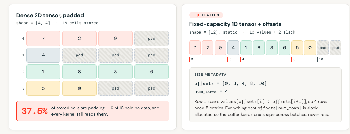
But we can't just do this arbitrarily. Simply passing the 1D tensor to the model may be acceptable for pretraining, but for finetuning we need to ensure that, within an example, tokens only attend to tokens in the same example. To fix this we have to pass in the correct example position_ids to the model. In turn the model will pass these to the fused attention kernels, and it will apply the correct attention mask. If you look at the example code you can see how we compute the needed inputs to make this work.
With this simple looking change, our training time goes from 2 hours 5 minutes to 1 hour and 17 minutes. There are two reasons why:
- The primary reason is that this packing increases the number of sequences per batch and reduces the total number of batches by approximately 36%. Note that this depends on the distribution and length of examples in your dataset.
- A secondary reason is that the flash-linear-attention kernels need to be just-in-time compiled for each input shape, and the shape was previously dynamic, leading to a few extra minutes of compilation.
Trade-off: this style of change does make the input pipeline more complex, and there's a high chance of introducing errors that impact model quality. But in this case the 36% savings are worth it. There are other techniques for reducing padding, such as keeping the original batching mechanism but sorting all inputs by length so that the padding is minimized; however this order may introduce unexpected correlation in adjacent samples, biasing the model.
Takeaways
- When training LLMs over a dataset with inputs shorter than your max trainable tokens (e.g. in this case 8192), efficiently packing data into batches can save a significant amount of time. For this dataset we saw a 1.6x improvement in training speed, taking our training time from 2 hours 5 minutes to 1 hour and 17 minutes.
Conclusions
In this post we showed how to 6x your training efficiency. It came down to three things: (1) first measuring what matters, not just GPU utilization but also where your model is spending time during training; (2) optimizing and fusing kernels, using known libraries like Flash Linear Attention; and (3) tailoring how batches of data are fed into the model.
To do this at scale you need a platform that makes the performant path the default. On AI Runtime many of these improvements are built in: the base environments bundle recent CUDA and Flash Attention, core metrics such as GPU utilization, temperature and health are tracked automatically, torch versions and the profilers are kept up to date, and reading data from Databricks is optimized through UCVolumeDataset. The recipe is reproducible end to end from the public cookbook referenced above.
Source: Reducing Qwen training time by 6x on AI Runtime, Bruce Fontaine and Pardis Beikzadeh, Databricks Blog, October 14, 2026. Figures and tables reproduced from the original post.
Source:Databricks Bloghttps://www.databricks.com/blog/reducing-qwen-training-time-6x-ai-runtime