Obstacle-Aware Autonomous Coverage and Navigation for Outdoor Robots

Paper: Obstacle-Aware Autonomous Coverage and Navigation for Outdoor Robots
Authors: Leonardo Gargani, Matteo Frosi, and Matteo Matteucci, Department of Electronics, Information and Bioengineering (DEIB), Politecnico di Milano
Publication: arXiv 2609.01384v2, 11 September 2026, CC BY 4.0, cs.RO
Paper: https://arxiv.org/abs/2609.01384
Code status: The authors did not release a public implementation of the complete system. The analysis checks the upstream Fields2Cover and opennav_coverage projects cited by the paper, but those repositories are not a reproduction of the author-built localization, behavior-tree, and field experiment stack.

1. Background: A Geometrically Valid Plan Is Not Yet a Field-Ready Mission

Solar farms, logistics yards, and large managed green areas increasingly use autonomous platforms for repetitive mowing, sweeping, inspection, and soil treatment. These tasks share a coverage-path-planning structure: a robot carries a tool of finite width and must sweep a bounded region without crossing known obstacles. Classical methods already provide mature geometric tools for decomposition, swath generation, route ordering, and path construction. Producing a polygon-following route is therefore not the only technical problem addressed here.

The harder problem is preserving mission reliability after the route leaves the planner. Outdoor robots move slowly, turn frequently, and operate for long periods. Wheel odometry accumulates yaw error in this regime. GNSS reception can degrade through multipath, obstruction, or a changing sky view. A geometrically short connector may not be compatible with the closed-loop controller. A newly observed pedestrian or temporary object may occupy several future goals. A long route may also require an energy-aware stop and a subsequent recovery or recharge cycle.

Prior work often optimizes these pieces separately. Coverage planning research studies swath orientation, headland turns, and travel length. Navigation frameworks such as Nav2 provide costmaps, controllers, recovery behaviors, and behavior trees. GNSS research studies global position and attitude estimation. Connecting such modules is not sufficient by itself because their inputs, failure modes, and time scales differ. A planner may reason in meters and route segments, whereas a controller needs feasible local goals and a localization filter must maintain a global frame for the entire mission.

The paper targets the gap between a geometrically valid route and a deployable field mission. It keeps the cell-decomposition and swath structure of Fields2Cover rather than deriving a new globally optimal coverage algorithm. Its contributions add a custom localization filter, three execution-oriented planning refinements, a behavior-tree mission layer, cost-aware handling of blocked goals, and autonomous docking.

The evaluation asks a deployment-oriented question: with one parameter set and no human intervention after site preparation, can the same stack complete routes over fields with different shapes, scales, and obstacle layouts? The paper reports mission completion, route duration, and an execution-focused coverage metric rather than benchmarking a planner on a standard synthetic dataset.

2. Problem Formulation and the Meaning of Coverage Efficiency

The target is a single differential-drive robot operating on predominantly planar outdoor terrain. The outer boundary is a polygon B, and a set O contains known obstacle polygons mapped during preparation. Obstacles that appear at runtime belong to a separate unknown set and are handled by the online navigation layer.

Each known obstacle is expanded by a safety margin and subtracted from the interior of the boundary. The admissible region is

$$\mathcal A=\operatorname{int}(\mathcal B)\setminus\bigcup_{i=1}^{m}O_i^\delta$$

where O_i^δ contains every point within distance δ of obstacle i. The margin δ is at least the robot footprint radius and may include additional clearance. In plain terms, the equation keeps the usable interior and removes every known obstacle together with its safety buffer.

The robot has working width w, adjacent swaths are spaced by d_s, and d_s is smaller than or equal to w. The difference w-d_s is deliberate overlap. For a path γ parameterized by arc length s, the area swept by the tool is

$$S(\gamma)=\bigcup_{s\in[0,L]}D_w\bigl(\gamma(s)\bigr)$$

Here D_w is the width-w band centered on the robot and orthogonal to its heading. This converts a one-dimensional route into the two-dimensional ground area actually treated by the tool.

Let γ_plan denote the planned route and γ_exec the executed route. Coverage efficiency is

$$\eta_c=\frac{\left|S(\gamma_{\mathrm{exec}})\cap S(\gamma_{\mathrm{plan}})\cap\mathcal A\right|}{\left|S(\gamma_{\mathrm{plan}})\cap\mathcal A\right|}$$

The numerator is the admissible planned area that the robot actually swept, while the denominator is the area the plan intended to sweep. Areas crossed twice count once. The metric deliberately isolates execution fidelity from route choice. A high value means the robot followed and treated the intended bands, not that the underlying plan is globally optimal or covers every part of the site that a user might regard as useful.

Mission success has a separate binary definition. After preparation, the robot must reach the route start, traverse the complete route, and complete the terminal phase, including docking when required, without human intervention. Success therefore measures the whole mission, while η_c measures the quality of coverage within a successful or unsuccessful run.

3. System Architecture and Platform

The system separates offline preparation and planning from online execution. Offline preparation records or imports a site boundary, builds obstacle polygons with clearance, and produces an admissible region. Fields2Cover then creates and orders swaths. Three refinements adapt the route to the controller and site layout. The output is a reusable route Σ, which can be executed repeatedly without replanning the entire site.

flowchart LR
    A[Record site perimeter] --> B[Load known obstacles]
    B --> C[Buffer obstacles and build free space]
    C --> D[Fields2Cover swaths and route]
    D --> E[Collinearity-aware resampling]
    E --> F[Straight connector intents]
    F --> G[20 Hz navigation execution]
    G --> H{Battery sufficient}
    H -->|Yes| I[Continue coverage]
    H -->|No| J[Return and dock]
    G --> K[Defer blocked goals]
    K --> G

Online, a two-level behavior tree supervises the route. A 20 Hz extended Kalman filter maintains the global pose. Local and global costmaps separate unknown-obstacle safety from known site structure. A Regulated Pure Pursuit controller follows a truncated local path at a nominal speed of 0.4 m/s. If energy is low or a mission fails, the mission tree invokes return-to-dock rather than relying on an operator to recover the platform.

The experimental platform is a differential-drive outdoor maintenance robot equipped with wheel encoders, a Unicore UM982 dual-antenna RTK-GNSS receiver, a Livox Mid-360 3D LiDAR, and a rear camera. A fixed GNSS base station provides georeferenced measurements. Coverage planning and navigation use a common metric frame, and all computation runs onboard without cloud services or remote processing.

The deployed planner uses boustrophedon swath ordering with a working width of 1.0 m and spacing of 0.9 m. Adjacent passes therefore overlap by 0.1 m. A differential-drive platform can rotate in place, so its effective minimum turning radius is zero. The paper can focus on waypoint density and connector clearance rather than continuous-curvature headland turns required by car-like agricultural vehicles.

4. Localization: Treating Heading as a Primary Mission State

The coverage tool is mounted laterally, so a yaw error changes the physical location of the treated band. Low-speed, turn-heavy operation makes wheel odometry a weak long-term heading source. The paper addresses this by fusing wheel odometry, GNSS position, measured dual-antenna yaw, and a fallback trajectory heading in a custom 12-state EKF.

The state vector contains position, Euler angles, body-frame linear velocity, and body-frame angular velocity:

$$\boldsymbol{\xi}=[x,y,z,\phi,\theta,\psi,v_x,v_y,v_z,\omega_x,\omega_y,\omega_z]^{\top}$$

For planar coverage, z and the vertical motion states do not directly affect the ground sweep. GNSS position primarily corrects x and y, dual-antenna orientation corrects ψ, and wheel odometry primarily corrects forward and yaw velocity. The larger state retains a general 3D attitude representation while supporting the planar navigation frame used in these experiments. The paper does not report separate ground-truth attitude errors, so this state design should not be read as a validation of steep or highly uneven terrain.

Prediction uses a constant-velocity model. Position is updated by rotating body-frame velocity into the global frame, attitude is updated through a mapping from body angular velocity to Euler rates, and covariance is propagated with the Jacobian of the nonlinear transition:

$$\mathbf P_{k+1}^{-}=\mathbf F_k\mathbf P_k^{+}\mathbf F_k^{\top}+\Delta t\mathbf Q$$

The process-noise matrix Q is block diagonal with separate entries for position, orientation, linear velocity, and angular velocity. A larger Q allows the estimate to react faster to measurements but also lets uncertainty grow more aggressively when measurements are missing.

Model gating protects each measurement update. For measurement z_k and predicted measurement h(ξ̂_k^-), the innovation and innovation covariance are

$$\boldsymbol\nu_k=\mathbf z_k-\mathbf h(\hat{\boldsymbol\xi}_k^{-}),\qquad \mathbf S_k=\mathbf H_k\mathbf P_k^{-}\mathbf H_k^{\top}+\mathbf R_k$$

The update is accepted only when the squared Mahalanobis distance is below a sensor-specific threshold:

$$d_k^2=\boldsymbol\nu_k^{\top}\mathbf S_k^{-1}\boldsymbol\nu_k\lt\tau_s^2$$

The GNSS position and measured-yaw threshold is 5, while the odometry twist threshold is 10. A gate is not a fixed Euclidean limit. It normalizes the residual by the filter's current uncertainty, so the same physical displacement can be accepted when uncertainty is high and rejected when the prediction is very confident. Angular innovations are wrapped to [-π, π] before gating.

When dual-antenna yaw is unavailable, the system estimates heading from successive accepted GNSS positions. A new point enters the window only after the robot has moved at least 0.3 m, and the window retains at most five such points. Directions β_j between accepted points are combined with a circular mean:

$$\hat\psi_k=\operatorname{atan2}\left(\sum_j\sin\beta_j,\sum_j\cos\beta_j\right)$$

Circular averaging avoids the discontinuity of an ordinary mean near ±π. The derived heading is used only when the directional dispersion in the window stays below 0.1. If neither direct nor trajectory-derived heading is valid, the filter skips the yaw update and propagates attitude until a valid source returns.

Localization parameter	Value	Role
Position process noise Qp	(0.05, 0.05, 0.05)	Growth of position uncertainty
Attitude process noise Qrpy	(0.03, 0.03, 0.03)	Growth of roll, pitch, and yaw uncertainty
Linear velocity noise Qv	(0.025, 0.025, 0.04)	Body-frame velocity uncertainty
Angular velocity noise Qω	(0.01, 0.01, 0.02)	Body-frame angular-rate uncertainty
GNSS gate τGNSS	5	Reject abnormal position and measured-yaw updates
Odometry twist gate	10	Tolerate short-term chassis dynamics
Heading-window displacement δp	0.3 m	Avoid heading estimation from GNSS-scale noise
Heading-window size N	5	Balance smoothness and turn response
Direction consistency Vthr	0.1	Reject unstable trajectory heading

The strength of this design is not the number of states. It is the explicit source hierarchy and separate gating. Dual-antenna yaw works during slow motion and in-place rotation, trajectory heading supplies a degraded-mode fallback, and wheel odometry supplies high-rate velocity information. The filter does not collapse all measurements into an undifferentiated pose update.

5. Coverage Planning: Preserve the Geometry, Repair the Execution Interface

In the paper's configuration, Fields2Cover offsets the boundary inward, fills the interior with parallel swaths, orders the swaths, and connects consecutive swaths with motion primitives. The authors keep this pipeline as the geometric backbone and identify three mismatches with their closed-loop controller and field layouts.

5.1 Collinearity-aware resampling

Raw planning output has dense points at turns but may leave straight swaths with very few intermediate poses. Uniform resampling repairs the straight sections but dilutes turn density. The method therefore measures local bending before changing waypoint spacing.

For an internal vertex p_i, define the skipped chord c_i=p_i+1-p_i-1 and incoming step d_i=p_i-p_i-1. The collinearity angle is

$$\alpha_i=\arccos\frac{c_i\cdot d_i}{\lVert c_i\rVert\lVert d_i\rVert}$$

The angle is near zero on a straight run and grows with the sharpness of local bending. The algorithm first enforces minimum and maximum spacing, removes near-collinear internal vertices, and then re-interpolates any remaining long segments.

1. Start with the first waypoint and compare each original point with the last accepted point.
2. Split distances above 0.5 m, keep points separated by at least 0.1 m, and reject points closer than the minimum.
3. Drop internal vertices whose angle is at most 0.01 degrees.
4. Insert evenly spaced points in any remaining segment longer than 0.5 m.

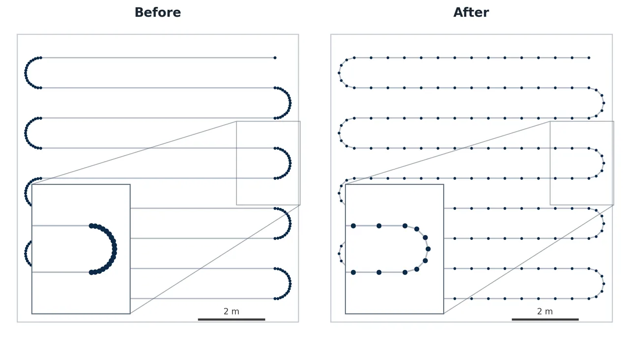
Figure 3(a): The original route is on the left and the resampled route is on the right. Straight sections gain uniform goals while turn geometry remains densely sampled.

The refinement changes more than the number of stored poses. Sparse goals can let a pure-pursuit controller cut a long swath or accumulate lateral error. Excessively dense goals can cause frequent goal switches and hesitation at headlands. Constraining spacing to a 0.1 to 0.5 m band while retaining turn points aligns the goal stream with a 0.4 m/s differential-drive controller and a 5 m path horizon.

5.2 Obstacle-aware straight connectors

Fields2Cover swaths observe the inflated obstacle boundary, but the native connector routine is separate and may cross an inflated obstacle. The authors disable native connector generation and replace each inter-swath transition with a straight goal-to-goal intent.

That line is not a committed trajectory. It fixes the ordering structure between swaths. At runtime, the global planner uses the known-obstacle costmap to route around static structure, while the local costmap uses live LiDAR to enforce clearance from unknown obstacles. If a connector is blocked, the goal manager defers affected goals and lets the robot continue with reachable work.

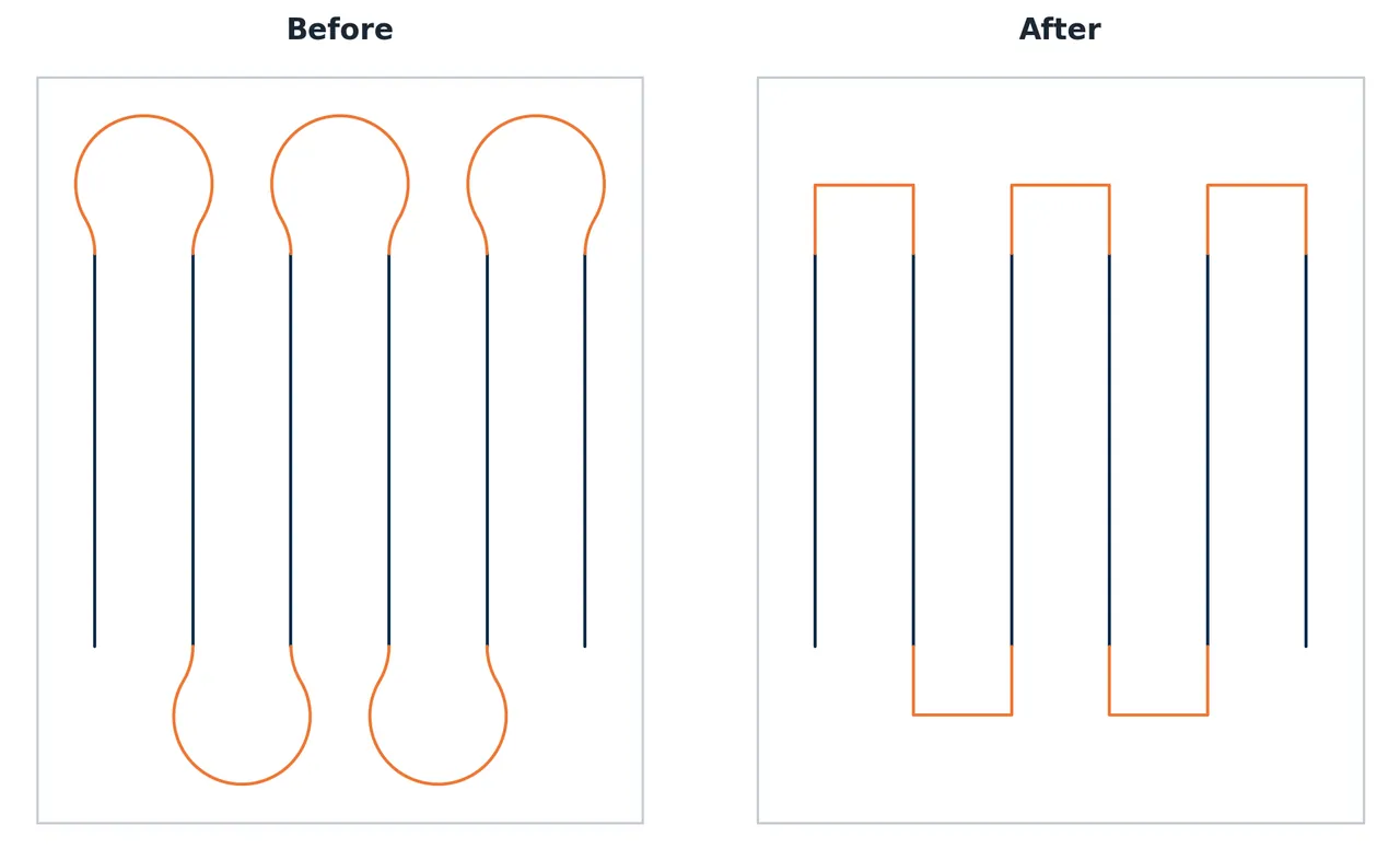
Figure 3(b): The native looping connectors are replaced by straight inter-swath intents, leaving the navigation layer to realize an obstacle-free motion.

This division of responsibility improves field flexibility but weakens offline guarantees. The route no longer contains a fully checked drivable connection for every unknown-obstacle configuration. Known obstacles remain in the global map, but an obstructed connection depends on online planning, goal deferral, and eventual recovery. This is an intentional system tradeoff rather than a property that can be inferred from geometric completeness alone.

5.3 Layout-aware obstacle clustering

Densely packed small obstacles can produce narrow gaps that are geometrically free but unsafe or infeasible for the robot. The method rasterizes the obstacle layer, dilates occupied pixels with a rectangular structuring element, and extracts outer contours as merged obstacle polygons. The mask is wider across the driving direction and sized from the required robot clearance.

If the gap between two obstacles is smaller than the mask width, they become one polygon. The corresponding narrow passage disappears from the admissible region. Because only narrow gaps are absorbed, the lost free area is limited, while the route planning problem becomes topologically simpler and less likely to generate fragile transitions.

5.4 Planning and execution parameters

Stage	Parameter	Value
Coverage planning	Working width w	1.0 m
Coverage planning	Swath spacing ds	0.9 m
Coverage planning	Minimum waypoint spacing dmin	0.10 m
Coverage planning	Maximum waypoint spacing dmax	0.50 m
Coverage planning	Collinearity threshold αthr	0.01 degrees
Online execution	Goal horizon K	4
Online execution	Goal pruning radius	0.85 m
Online execution	Controller path truncation	5 m
Online execution	Goal cost threshold cmax	10
Online execution	Maximum postponements rmax	3
Online execution	Position and heading tolerance	0.5 m, 0.5 rad

The values are coupled. A pruning radius of 0.85 m exceeds the maximum waypoint spacing of 0.5 m, so the robot does not stop at every goal. It remains below the 0.9 m swath spacing, which reduces the chance of marking a goal on the adjacent pass as complete. A four-goal horizon and a 5 m controller truncation keep each planning cycle bounded regardless of the full route length.

6. Online Execution: Behavior Trees Carry Mission Autonomy

A compact mission tree checks energy, extracts route goals, undocks, hands the route to navigation, and docks at the end. A lower navigation tree first drives to the route start with a single-goal horizon, then enters a recovery-wrapped plan-and-follow loop.

The recovery subtree escalates through bounded actions: clear the local costmap, clear the global costmap, rotate in place to refresh perception, wait briefly for a temporary obstacle, and back up a short distance. The order starts with low-disturbance actions and proceeds to a change of robot position. This treats stale perception, temporary blockage, local minima, and physical entrapment as different failure cases instead of invoking one generic replanning action.

Unknown obstacles are handled by goal management as well as replanning. Because coverage goals are densely sampled, an obstacle can overlap several future goals. Replanning to the next blocked pose may therefore remain unsuccessful. Before each planning cycle, the supervisor examines the local-costmap cost of upcoming goals. A goal above threshold 10 is moved to the back of the queue, allowing the robot to work on reachable goals first. It is retried when it reaches the front and dropped only after three postponements.

The method turns the route into a priority-ordered set of work targets without changing the offline coverage geometry. A temporary pedestrian causes deferral rather than mission termination. Once the rolling local map clears, the goal may become reachable again. A persistent blockage eventually consumes the postponement budget and is dropped so the rest of the mission can proceed.

Docking uses the same mission supervisor. The robot navigates to a fixed staging pose in front of the dock, keeps an ArUco marker in the rear camera view, and estimates the relative marker pose for closed-loop alignment. A change in the power state confirms successful charging. Undocking reverses the alignment until the robot returns to the staging pose. Energy management is therefore part of the behavior tree rather than an external manual procedure.

7. Field Evaluation

The paper reports five real outdoor areas ranging from 168.0 to 1640.9 m². The set includes convex and non-convex boundaries with and without known obstacles. All runs use the same operating protocol and parameter set, and no human intervention is required after preparation. The authors also plan a simulated 1.5 ha photovoltaic site, but that large-scale case is not executed by the real robot.

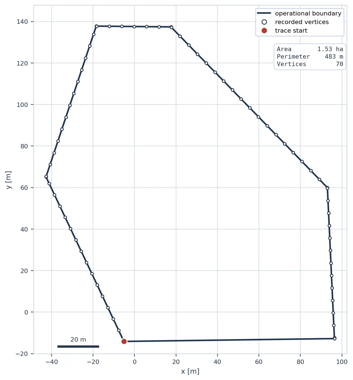
Figure 1: The robot records a site perimeter and establishes a metric admissible region. The resulting site model can be reused for repeated missions.

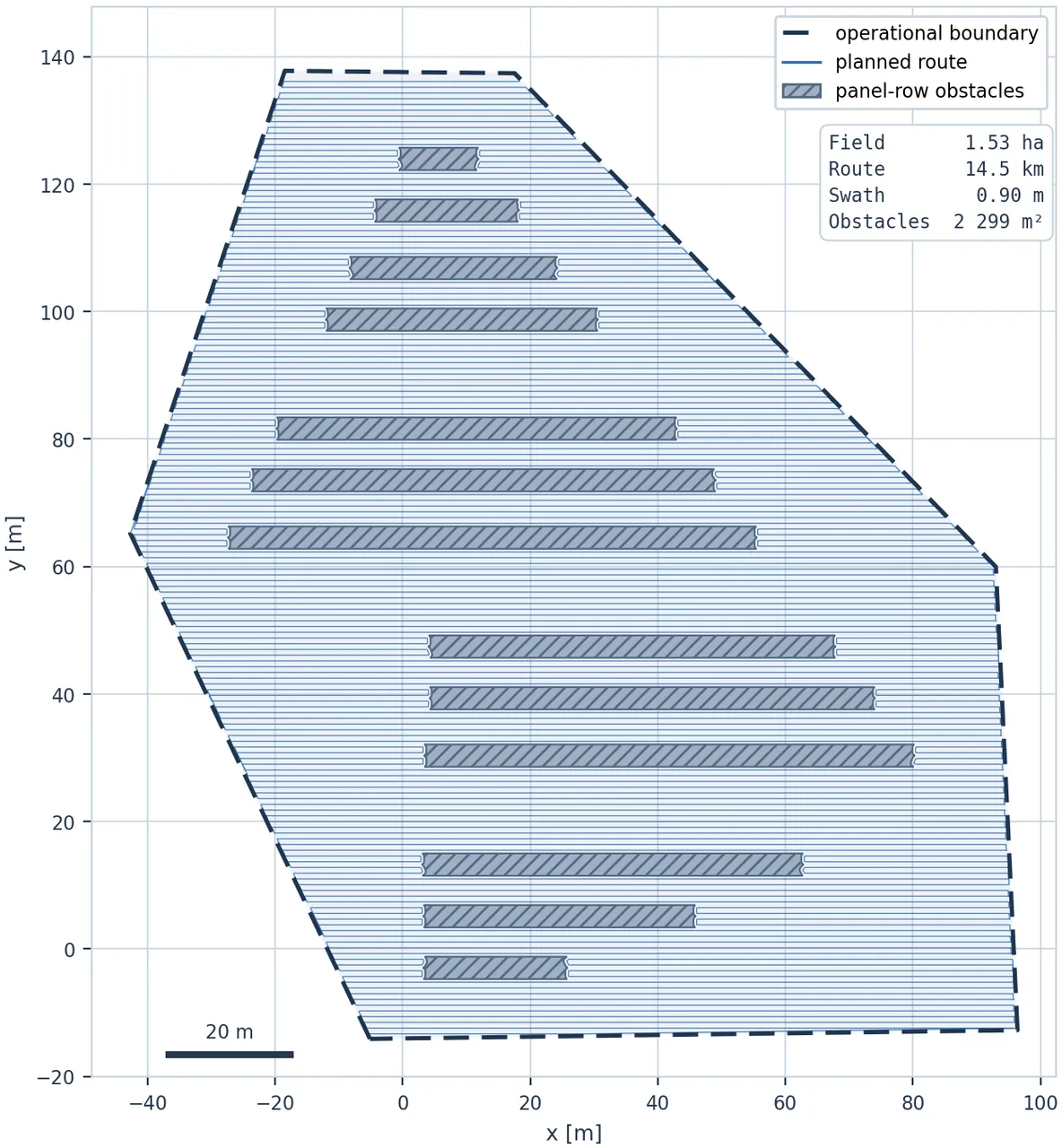
Figure 1: Parallel swaths are generated inside the admissible region and route around known obstacle footprints.

Seq.	Shape	Field m²	Planned m²	Route m	Obstacles m²	Duration min:s	Coverage
01	Convex	168.0	156.3	180.0	0.0	8:35	93.2%
02	Convex	196.1	190.6	221.2	0.0	10:12	94.2%
03	Non-convex	372.7	304.2	356.3	7.5	16:07	93.1%
04	Non-convex	948.2	711.9	837.2	65.2	36:15	94.9%
05	Convex	1640.9	1397.9	1614.1	98.5	68:37	96.1%

All five missions satisfy the paper's complete-route, no-intervention success criterion. Coverage efficiency varies by only three percentage points. The non-convex obstacle fields do not form a separate low-performance cluster, and the largest field records the highest efficiency. The planned area is smaller than the enclosed field because headlands, safety boundaries, and inflated obstacle footprints are not treated as coverage area.

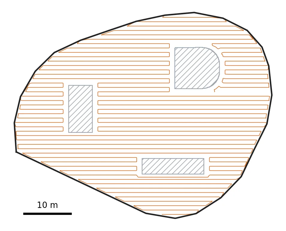
Figure 6: The planned route for the largest field. Parallel swaths are joined by straight intents, with clearance around the three known obstacles.

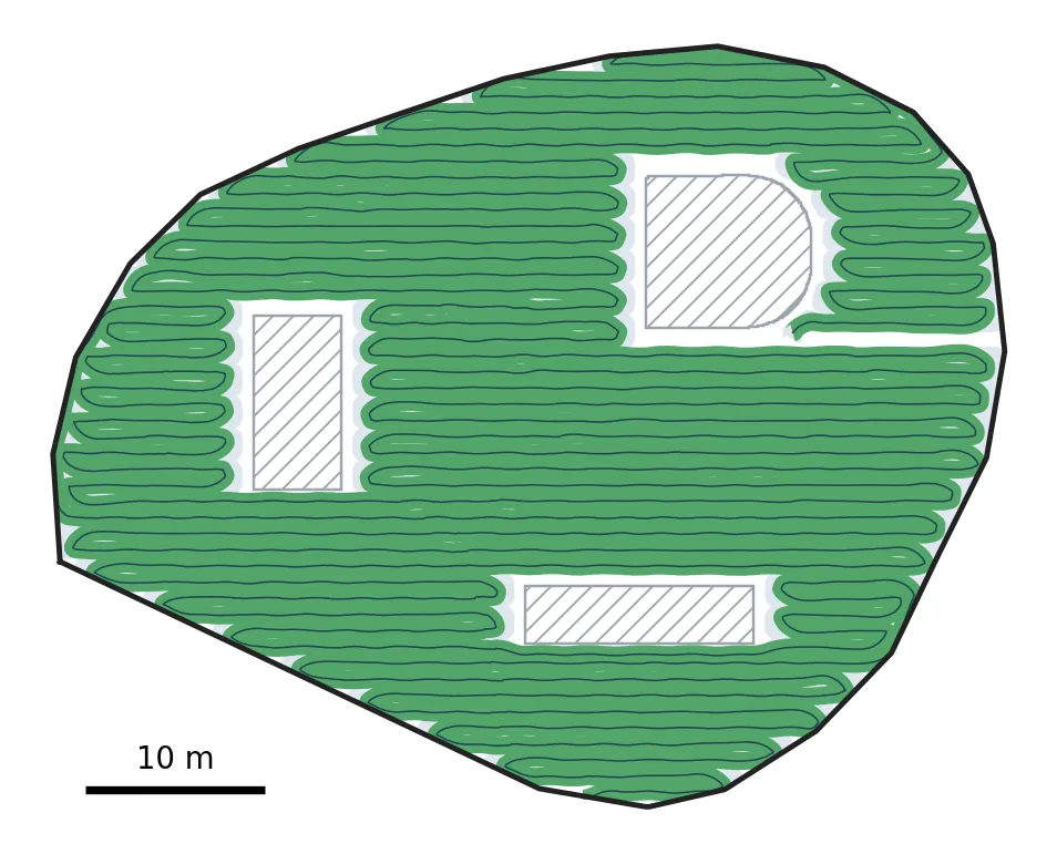
Figure 6: Executed sweep on the same site. The green area tracks the planned bands while leaving clearance at obstacle footprints and the boundary.

Route density provides a separate check on geometric efficiency. Across all five areas, the planned route is 1.15 to 1.18 m per planned square meter. The designed swath spacing alone implies about 1/0.9=1.11 m/m². Headland turns and inter-swath connections therefore add roughly 4% to 6% to the route. This ratio is stable across field size, polygon shape, and obstacle count, indicating that the connectors and boundary handling do not cause large route inflation in this test set.

The authors also introduce pedestrians and temporary objects. Live LiDAR observations cause the robot to slow, reroute, or defer blocked goals, and coverage resumes after the obstacle clears. The reported evidence for this scenario is qualitative. The paper does not count obstacle encounters, report minimum separation, quantify the number of postponed goals, or measure recovery latency. It therefore demonstrates that the execution path was exercised, not that the system has a measured real-world obstacle-avoidance success rate.

8. What the Results Support and What They Leave Open

The strongest result is not the maximum efficiency of 96.1%. It is the narrow 93.1% to 96.1% range across five sites whose route lengths vary from 180 to 1614 m. If the integrated stack were highly sensitive to polygon shape or known obstacles, coverage fidelity would be expected to degrade as the task scales. The observed range supports the claim that localization, goal density, and online navigation behave coherently within these test conditions.

Mission completion is a second important signal. Long-duration coverage exposes localization drift, recovery failures, and energy-management gaps that a short point-to-point navigation test may not reveal. Completing routes from under nine minutes to more than an hour without an operator restart is evidence of system-level feasibility.

The experiment does not include an ablation or baseline comparison. A reader cannot determine how much coverage or time would be lost by removing dual-antenna yaw, reverting the resampling, restoring native connectors, or disabling goal postponement. The reported metric compares the full system with its own plan, not the proposed refinements against standard coverage and Nav2 pipelines. The paper therefore supports integrated feasibility, but not the stronger causal claim that each refinement is necessary or optimal.

Each site is executed once, and no confidence intervals or repeated-run distribution are reported. Differences between sites cannot be separated from weather, GNSS geometry, temporary obstacles, and run-to-run variation. There is also no independent high-precision truth for RTK position and heading. Coverage efficiency is computed from the same overall localization and tool-width model used for execution, so a slow global pose drift could affect both the robot control and the evaluation.

The 1.5 ha photovoltaic-site experiment is planning-only. It shows that the Fields2Cover workflow can represent a site larger than any physical test area, but it does not validate an hour-scale mission, recharge interruption, local sensing, or docking at that scale. The largest executed field is 1640.9 m², roughly 0.164 ha, an order of magnitude smaller.

9. Code and Implementation Audit

The paper does not publish the author-built ROS 2 packages, 12-state EKF, mission behavior trees, or complete experimental configuration. A search based on the exact title and authors did not identify an official repository. External readers therefore cannot inspect how the filter, goal postponement state machine, docking sequence, or recovery budget are implemented.

The upstream dependencies are publicly available and were checked for architectural context. Fields2Cover examples confirm the expected headland, swath, route-ordering, and motion-primitive stages, so the paper's claim that it extends a mature geometric planner is consistent with the public library. opennav_coverage provides a Nav2-compatible route toward exposing coverage as a task server and behavior-tree action. Its public examples are much narrower than the full article system and do not supply the custom localization stack, controller-specific resampling, goal-level unknown-obstacle management, docking, or field evaluation. These repositories clarify the dependencies but are not a substitute for the authors' source code.

For reproducible deployment, the most valuable missing artifacts would be the measurement models and gate configuration of the EKF, the GNSS heading-window logic, the interface between route goals and the Nav2 behavior tree, and the exact goal-deferral state machine. Without them, an external team can reconstruct the broad architecture but cannot establish that its implementation matches the behavior reported in the paper.

10. Limitations

The authors explicitly identify two future directions. First, the localization stack is not designed to remain globally accurate through severe GNSS degradation or a long complete outage. The EKF can propagate through short gaps and the trajectory-direction fallback can replace measured yaw, but a prolonged loss of absolute observations still requires another source such as vision, LiDAR map matching, or learned relative localization. Second, the system addresses only one robot. Multi-robot area partitioning, communication interruption, inter-robot avoidance, and fleet charging schedules remain outside the study.

The independent limitations are experimental scale and repeatability. One platform and five single runs do not estimate long-term reliability. The operational value of coverage robots depends on tail events accumulated over many missions: a sudden GNSS jump, a pedestrian stopped on a swath, wheel slip, a low battery near a difficult obstacle, or a failed charging contact. None of these rates are reported.

The coverage metric also does not fully evaluate plan quality. η_c can be high when the executed area closely matches a plan that itself omits useful ground. A more complete evaluation should report effective site area, planned coverage completeness, executed coverage completeness, route length, duration, and intervention count. It should compare the integrated system with native Fields2Cover and a conventional Nav2 coverage baseline under the same sites.

Connector feasibility is delegated to the online planner. The design deliberately turns straight lines into goal intents, which makes the physical system more flexible but weakens offline geometric guarantees. The five trials show that the online layer can absorb the resulting uncertainty, but they do not report worst-case detour length, planning latency, or the number of dropped goals in dense clutter.

11. Conclusion

The paper is best understood as an integrated field-robotics system rather than a single planning algorithm. It connects global localization, admissible-area preparation, geometric coverage planning, controller-oriented route refinement, behavior-tree supervision, reactive obstacle handling, and autonomous docking. Five real sites show that the complete chain can run continuously without human intervention. Coverage efficiency remains between 93.1% and 96.1%, and route density stays between 1.15 and 1.18 m/m² as the field grows from 168 to 1641 m².

The next step should be a structured ablation and fault study. Removing dual-antenna yaw, collinearity-aware resampling, connector replacement, and goal postponement one at a time would quantify their effects on mission completion, coverage, recovery count, route length, and energy. A second direction is to add vision or LiDAR localization for extended GNSS denial and then execute repeated missions on a genuinely large photovoltaic site.

The hard part of outdoor coverage is not drawing a route. It is keeping localization, geometry, control, and mission supervision aligned with that route through tens of minutes of real disturbance.