PAPER DEEP DIVE
GSQ: Highly-Accurate Low-Precision Scalar Quantization for LLMs via Gumbel-Softmax Sampling
Quantization has become a standard tool for efficient LLM deployment, especially for local inference, where models are now routinely served at 2-3 bits per parameter. The state of the art is currently split into simple scalar quantization techniques, such as GPTQ or AWQ, which are widely deployed but plateau in accuracy at 3-4 bits per parameter (bpp), and "second-generation" vector- or trellis-quantized methods, such as QTIP, GPTVQ and AQLM, which push the accuracy frontier but are notoriously hard to implement and to scale. In this paper, we ask whether this gap is fundamental, or whether a carefully optimized scalar quantizer can recover most of it. We answer in the affirmative, by introducing GSQ (Gumbel-Softmax Quantization), a post-training scalar quantization method which jointly learns the per-coordinate grid assignments and the per-group scales using a Gumbel-Softmax relaxation of the discrete grid. GSQ matches the cardinality of the relaxation to the small number of levels available in the target bit-width regime (e.g., 3-8 levels for ternary and 3 bpp, respectively), making optimization tractable. Practically, on the standard Llama-3.1-8B/70B-Instruct models, GSQ closes most of the gap between scalar quantization and the QTIP frontier at 2 and 3 bits, while using a symmetric scalar grid with group-wise quantization, and thus remains compatible with existing scalar inference kernels. We further show that the same discrete-assignment optimization can be applied to practical GGUF K-Quant checkpoints: starting from publicly released GGUF models, GSQ improves accuracy while projecting the result back into the same deployment format. Finally, GSQ scales to trillion-scale Mixture-of-Experts models such as Kimi-K2.5, where vector-quantized methods are difficult to apply. The source code is publicly available at https://github.com/IST-DASLab/GSQ.
Authors: Alireza Dadgarnia, Soroush Tabesh, Mahdi Nikdan, Michael Helcig, Eldar Kurtić, Maximilian Kleinegger, and Dan Alistarh
Paper: arXiv:2604.18556 Code: IST-DASLab/GSQ Topics: LLMs, post-training quantization, low-bit inference, GGUF, mixture-of-experts
One-sentence summary: GSQ treats low-bit scalar quantization as a differentiable discrete assignment problem, recovering much of the accuracy gap to vector quantizers without abandoning the kernels and deployment formats that make scalar quantization practical.
The deployment split between scalar and vector quantization
Large language models now strain memory capacity, memory bandwidth, interconnect, and serving budgets even when they are used only for inference. Quantization is no longer a peripheral compression trick. It determines how many weights fit on an accelerator, how many concurrent requests a service can hold, and whether a capable model can run locally on a workstation or robot platform.
The current low-bit landscape is split into two broad families. GPTQ, AWQ, and related scalar methods assign each weight to a small integer grid with a group-wise scale. Their advantage is systems compatibility. They map onto mature low-precision matrix kernels, support mixed bit allocation, and require no learned codebook lookup at inference time.
Vector and trellis quantizers such as QTIP, GPTVQ, and AQLM are more expressive. They encode relationships among multiple weights through codebooks or structured lattices, which can preserve more model quality at the same average bit rate. That gain comes with specialized decoding, harder training, and more difficult integration into standard serving stacks, especially for trillion-parameter mixture-of-experts models.
The paper asks whether the apparent scalar-versus-vector gap is largely an optimization gap. A scalar grid has fewer degrees of freedom than a codebook, so some gap must be fundamental. Yet standard scalar post-training methods also make a restrictive assumption: they decide most grid assignments through a local layerwise procedure and rarely revisit the full discrete choice under a richer objective.
GSQ attacks that second source of error. It keeps the final representation as ordinary symmetric scalar quantization, but gives each coordinate trainable logits over legal grid choices. A Gumbel-Softmax relaxation turns those choices into differentiable soft samples during optimization. The logits and group scales are learned jointly, then hardened with argmax when the model is exported.
This framing is especially useful at two and three bits. The number of candidate levels remains small enough for a probabilistic relaxation, while the penalty for a poor discrete assignment is severe. The method also connects naturally to already-quantized artifacts. A public GPTQ or GGUF checkpoint can serve as the warm start, and the optimization can improve its assignments while preserving the deployed format.
Problem formulation
Let $f(\cdot;\mathbf{w})$ denote a linear layer, Transformer block, expert, or larger model parameterized by weights $\mathbf{w}$. Given calibration inputs $\mathbf{x}$, quantization seeks a constrained weight vector that preserves the function output as closely as possible. The paper uses a Frobenius reconstruction objective:
$$\hat{\mathbf{w}}=\arg\min_{\bar{\mathbf{w}}}\left\lVert f(\mathbf{x};\bar{\mathbf{w}})-f(\mathbf{x};\mathbf{w})\right\rVert_F^2\quad\text{s.t.}\quad\bar{\mathbf{w}}\in\mathcal{C}.$$
The constraint set is the source of difficulty. It contains discrete grid points, masks, or signs, so ordinary gradient descent cannot directly differentiate through the final selection. A common approximation is to optimize continuous scales after applying a fixed rounding rule, but that separates the continuous and discrete parts of the problem. GSQ instead keeps a probability distribution over legal candidates during training.
For ternary quantization, the constraint can be written as a product of a shared scale, a zero-one mask, and a sign vector:
$$\mathcal{C}_{\text{ternary}}=\left\{\bar{\mathbf{w}}\mid\bar{\mathbf{w}}=s\cdot\mathbf{m}\odot\mathbf{b};\ s\in\mathbb{R},\ \mathbf{m}\in\{0,1\}^d,\ \mathbf{b}\in\{-1,1\}^d\right\}.$$
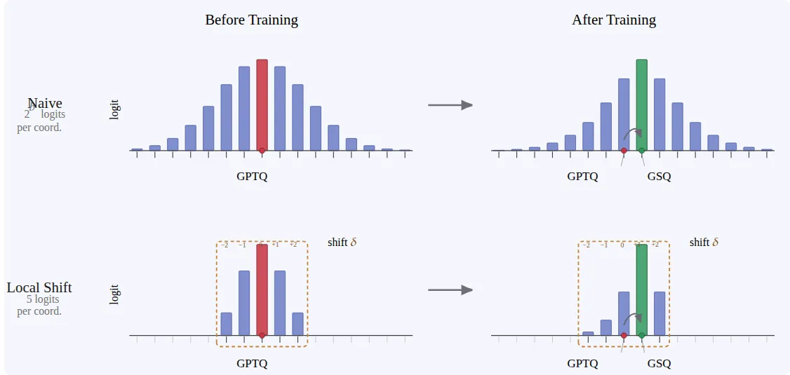
Each coordinate therefore needs two binary decisions: zero versus nonzero, and positive versus negative. A naive categorical parameterization would carry four logits per coordinate. The implementation exploits the equivalence between a two-class softmax and a sigmoid so that each binary decision can be represented with one scalar logit.
Method: differentiable grid assignment
GSQ starts from a strong discrete solution rather than random weights. For Llama experiments, GPTQ supplies the initial grid assignment and group scales. For GGUF experiments, a public K-Quant checkpoint supplies the starting structure. The method then improves that starting point under a block-level or expert-level reconstruction objective.
In the ternary case, the GPTQ mask and sign decisions initialize two sets of logits. Isotropic Gaussian noise is added before training so that the warm start guides the search without becoming an irreversible hard constraint:
$$\boldsymbol{\ell}=\sigma_{\mathrm{init}}\left(\boldsymbol{\epsilon}+\alpha\boldsymbol{\ell}_{\mathrm{GPTQ}}\right),\qquad\boldsymbol{\epsilon}\sim\mathcal{N}(\mathbf{0},\mathbf{I}).$$
Here $\alpha$ controls how strongly the GPTQ assignment dominates the injected noise, and $\sigma_{\mathrm{init}}$ controls the logit magnitude. A zero GPTQ weight still needs a usable sign logit because the mask may flip during optimization and activate the sign branch later.
For general $b$-bit scalar quantization with a full grid, the constraint is:
$$\mathcal{C}_{b\text{-bit}}=\left\{\bar{\mathbf{w}}\mid\bar{\mathbf{w}}=s\cdot\mathbf{q};\ s\in\mathbb{R},\ \mathbf{q}\in\mathcal{G}_b^d\right\},\qquad\lvert\mathcal{G}_b\rvert=2^b.$$
At two bits, the paper uses $\mathcal{G}_2=\{-2,-1,0,1\}$. The grid is asymmetric when viewed with a positive scale, so the scale itself is allowed to be negative. This preserves the ability to represent either orientation while retaining a symmetric scalar format in the deployed model.
The exponential candidate count becomes an engineering problem at three and four bits. The method could assign one logit per grid value per coordinate, but the temporary memory would scale as $d\cdot2^b$. The paper instead introduces a local-shift representation for widths above two bits. Each coordinate selects one of five relative moves around its initialized grid index:
$$q_i=(\mathcal{G}_b)_{\operatorname{clip}(j_i^0+\delta_i,1,2^b)},\qquad\delta_i\in\{-2,-1,0,1,2\}.$$
The index $j_i^0$ comes from the GPTQ or GGUF initialization. The learned variable is the shift $\delta_i$, not the absolute grid value. This reduces the auxiliary parameter count from $d\cdot2^b+1$ to $5d+1$. It also encodes an empirical assumption: after a good warm start, most useful corrections are local rather than long jumps across the whole grid.
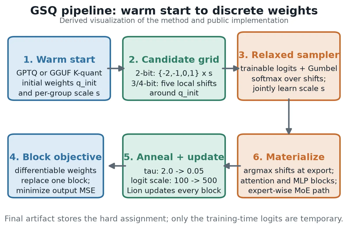
At each optimization step, Gumbel noise is added to the candidate logits. The perturbed logits are normalized at temperature $\tau$, with a separate logit scale $\kappa$, and the resulting probabilities form a soft candidate:
$$p_i=\frac{\exp\left((\kappa\ell_i+g_i)/\tau\right)}{\sum_{j=1}^{n}\exp\left((\kappa\ell_j+g_j)/\tau\right)},\qquad\tilde{d}=\sum_{i=1}^{n}p_i d_i.$$
Training begins at temperature 2.0 so that gradients can flow through multiple candidates. The temperature is annealed to 0.05 while the logit scale rises from 100 to 500. This schedule moves the relaxation from broad exploration toward an almost discrete distribution. The exported model does not use the soft expectation; it fixes the highest-logit candidate with a hard argmax.
The group scale is optimized jointly with the assignment logits. This matters because a change in discrete values alters the optimal step size, while a change in scale alters the relative cost of neighboring grid points. GSQ therefore differs from methods that first quantize each layer and only later tune a small set of continuous parameters. Both the discrete decision and the continuous scale participate in the same reconstruction loss.
Temperature annealing creates a known optimization hazard. When one logit dominates, the softmax approaches one-hot and its Jacobian can become extremely small. The appendix derives the bound:
$$\left\lVert\nabla_{\mathbf{a}}\ell(y)\right\rVert_{\infty}\leq\frac{(K-1)G}{\tau}e^{-\Delta/\tau}.$$
Here $K$ is the number of candidates, $\Delta$ is the gap between the largest and second-largest logit, and $G$ bounds the loss gradient with respect to the probability vector. Saturation therefore suppresses updates exponentially as the gap grows. The authors use Lion rather than relying on a large AdamW epsilon. Lion remains less sensitive to the vanishing-gradient regime produced by their annealing schedule.
The training objective is block level by necessity. A forward pass replaces one attention block, MLP block, or expert group with its current soft-quantized weights and measures the resulting output error. Gradients flow back to the logits and scale. Mini-batch gradient accumulation has a second benefit beyond memory reduction: because Gumbel noise is resampled in each forward pass, averaging across micro-batches lowers sampling variance.
flowchart TD
  A["GPTQ or GGUF warm start"] --> B["Group scales and initial grid indices"]
  B --> C["Full grid or five local shifts"]
  C --> D["Trainable assignment logits"]
  D --> E["Gumbel-Softmax soft sample"]
  E --> F["Replace one block and measure output error"]
  F --> G["Lion updates logits and scales"]
  G --> D
  D --> H["Anneal temperature and logit scale"]
  H --> I["Hard argmax assignment"]
  I --> J["Export in the original scalar format"]
The block schedule follows model structure. Dense Llama models are optimized in attention and MLP phases. Kimi-K2.5, a trillion-parameter mixture-of-experts model, is optimized expert by expert while shared experts and vision components remain in their original representation. This bounds the number of auxiliary parameters that must be resident at once and makes the method applicable to a model for which full-model codebook training would be impractical.
Two compact excerpts from the public repository show how the paper maps to code. The integer quantizer constructs the five local shifts and masks candidates outside the legal grid:
Source: src/quantization/gumbel_quantizer_int.py, constructor, lines 16 to 22.
self.shift_values = torch.tensor([-2.0, -1.0, 0.0, 1.0, 2.0])
cand = self.init.unsqueeze(0) + self.shift_values.view(-1, 1, 1)
self.valid_shift_mask = (cand >= self.min_grid) & (cand <= self.max_grid)
The forward path applies Gumbel noise, temperature scaling, the weighted shift, and the group scale in one differentiable computation:
Source: src/quantization/gumbel_quantizer_int.py, GumbelSoftmaxFunction.forward.
noise = -torch.log(-torch.log(u + eps) + eps)
soft_quant = F.softmax((masked_logits * ctx.scale + noise) / ctx.temperature, dim=0)
soft_output = (soft_quant * shift_values.view(-1, 1, 1)).sum(dim=0)
output = (init + soft_output) * scale_per_col
The original appendix figure isolates the parameterization itself. The upper row shows a full set of logits over the grid; the lower row shows five local shifts around the GPTQ assignment before and after training. The figure explains the candidate-count reduction but does not describe the whole optimization pipeline, which is why the derived diagram above is used for the end-to-end view.
Llama experiments and inference speed
The main controlled comparisons use Llama-3.1-8B-Instruct and Llama-3.1-70B-Instruct. Baselines include GPTQ, QuIP, EfficientQAT, QTIP, and PV-Tuning. Evaluation covers ARC-Challenge, ARC-Easy, HellaSwag, PIQA, and WinoGrande, with their average used as the headline zero-shot score. Llama calibration uses FineWeb-Edu with 4096 sequences of 4096 tokens for 20 epochs.
At two bits, GSQ improves substantially over the strongest scalar baseline. On Llama-8B it reaches 68.55, which is 4.76 points above EfficientQAT at 63.79, while remaining 1.33 points below QTIP at 69.88. On Llama-70B it reaches 75.57, 4.14 points above EfficientQAT, 1.68 below QTIP, and 0.70 below PV-Tuning. The scalar format is therefore competitive but not universally superior to codebook methods.
| Method | 8B bpp | 8B average | 70B bpp | 70B average |
|---|---|---|---|---|
| FP16/BF16 | 16.00 | 73.71 | 16.00 | 78.99 |
| GPTQ | 2.25 | 37.53 | 2.25 | 57.38 |
| EfficientQAT | 2.25 | 63.79 | 2.25 | 71.43 |
| QTIP | 2.00 | 69.88 | 2.00 | 77.25 |
| PV-Tuning | 2.27 | 69.83 | 2.07 | 76.27 |
| GSQ | 2.13 | 68.55 | 2.13 | 75.57 |
The three-bit comparison follows the same ordering. GSQ reaches 72.32 on Llama-8B and 77.99 on Llama-70B, making it the strongest scalar method in both columns. Ternary GSQ on Llama-8B is also competitive with several higher-rate scalar baselines. These results matter because they show that the method is not only repairing the extreme two-bit regime; the discrete-assignment idea remains useful when the grid has more levels.
Standard scalar layers make nonuniform bit allocation straightforward. The paper reports average 2.62 and 2.37 bits on Llama-70B with averages of 77.50 and 77.40, and 2.37 bits on Llama-8B with an average of 69.44. The point is not that a particular mixed schedule dominates every uniform setting. It is that GSQ can move along the accuracy-rate curve without changing the deployed scalar representation.
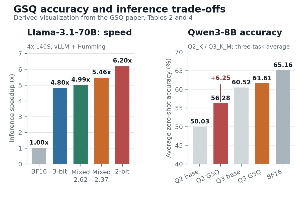
The end-to-end throughput experiment demonstrates why format compatibility matters. Llama-70B is served with vLLM and Humming kernels on four NVIDIA L40S GPUs. BF16 produces 60.3 output tokens per second per GPU. Uniform two-bit GSQ reaches 374.0, a 6.20x speedup. The 2.37 and 2.62 bit nonuniform configurations reach 5.46x and 4.99x. These are measured end-to-end serving results rather than arithmetic-operation estimates.
| Representation | Average bits per parameter | ShareGPT TPS/GPU | Speedup over BF16 |
|---|---|---|---|
| BF16 | 16.00 | 60.3 | 1.00x |
| Uniform 3-bit | 3.13 | 289.6 | 4.80x |
| Nonuniform | 2.62 | 301.1 | 4.99x |
| Nonuniform | 2.37 | 329.2 | 5.46x |
| Uniform 2-bit | 2.13 | 374.0 | 6.20x |
Kimi-K2.5 at trillion-parameter scale
Kimi-K2.5 is a trillion-parameter sparse mixture-of-experts model stored natively at four bits. GSQ quantizes only the nonshared expert weights to two bits, leaving shared experts and vision components unchanged. This selective scope reduces training cost and avoids applying aggressive quantization to paths that are not part of the intended experiment.
The calibration source is OpenThoughts, trained for 10 epochs. The reported average rate falls from 4.5 to 2.13 bits per parameter. AIME25 decreases from 95.33 to 93.00 and MATH500 rises slightly from 96.68 to 97.32. LiveCodeBench moves from 61.37 to 69.37. The last result reflects performance under the paper’s common evaluation pipeline, which the authors note differs from the model-card protocol.
GPQA Diamond falls from 89.29 to 76.57, a loss of 12.72 points. The authors connect this pattern to calibration composition. OpenThoughts emphasizes mathematics and code, which overlaps with AIME, MATH500, and coding tasks but covers less of the biology, chemistry, and physics knowledge in GPQA. A later Kimi-K2.6 run with a broader mixture narrows the science gap, but it changes the base model as well, so it is supporting evidence rather than a controlled ablation.
| Metric | Base | GSQ | Change |
|---|---|---|---|
| Bits per parameter | 4.50 | 2.13 | -2.37 |
| AIME25 | 95.33 | 93.00 | -2.33 |
| GPQA Diamond | 89.29 | 76.57 | -12.72 |
| LiveCodeBench | 61.37 | 69.37 | +8.00 |
| MATH500 | 96.68 | 97.32 | +0.64 |
| MRCR 0 to 8k | 95.37 | 97.81 | +2.44 |
| MRCR 8k to 16k | 77.81 | 85.75 | +7.94 |
| MRCR 16k to 32k | 69.19 | 74.41 | +5.22 |
| MRCR 32k to 64k | 57.10 | 53.73 | -3.37 |
| MRCR 128k to 256k | 46.04 | 44.91 | -1.13 |
Long context has a clear boundary. GSQ improves MRCR through 32k and loses only a small amount at 32k to 64k and 128k to 256k. The result supports the claim that aggressive weight quantization can retain substantial long-context behavior, but it also rules out the simpler claim that the model is uniformly preserved. Context length must be part of the deployment evaluation.
Training cost further qualifies the result. On eight H200 GPUs, Llama-8B takes 10 hours, Llama-70B takes 68 hours, and Kimi-K2.5 takes 24 hours. Kimi is larger than Llama-70B but does not quantize attention and uses fewer epochs. The comparison shows that runtime depends on the selected weight scope and schedule, not only model size. It also confirms that GSQ is an offline optimization rather than a near-instant conversion.
Improving existing GGUF checkpoints
GGUF K-Quant is one of the most important local inference formats. It defines block structures and mixed precision rules that are already supported by widely used runtimes. Rather than replacing those rules, GSQ treats a released Unsloth GGUF checkpoint as the initialization, optimizes its discrete assignment, and projects the result back into the same format.
On Qwen3-8B, GSQ raises Q2_K from 50.03 to 56.28 average accuracy, a gain of 6.25 points. Q3_K_M improves from 60.52 to 61.61. The larger gain at Q2_K is consistent with the idea that a weaker starting checkpoint leaves more room for assignment correction. Q2_K AIME25 rises from 38.67 to 52.00, and the number of generated AIME tokens falls from 0.64M to 0.58M.
| Format | AIME25 | GPQA Diamond | MMLU-Pro | Average |
|---|---|---|---|---|
| BF16 | 64.67 | 58.38 | 72.42 | 65.16 |
| Unsloth Q3_K_M | 56.67 | 54.65 | 70.23 | 60.52 |
| GSQ Q3_K_M | 59.00 | 55.15 | 70.67 | 61.61 |
| Unsloth Q2_K | 38.67 | 46.46 | 64.97 | 50.03 |
| GSQ Q2_K | 52.00 | 50.91 | 65.94 | 56.28 |
This does not mean that two-bit GGUF is solved. GSQ Q2_K remains 8.88 points below BF16 on the three-task average and 7.47 points below it on GPQA Diamond. The operational claim is narrower and more useful: within the same deployed format, better discrete assignments can recover a large part of the loss, especially for aggressive public checkpoints.
The GGUF result also exposes the method boundary. GSQ can choose only among assignments that the K-Quant format can represent. If a block parameterization is too coarse for a sensitive layer, the optimizer cannot invent the expressiveness of a vector codebook. GSQ improves existing formats; it does not remove their structural limits.
What the ablations establish
The optimizer ablation directly tests the saturation problem. AdamW reaches 61.84 average and Lion reaches 65.54, a 3.70 point difference. Lion is not merely a faster optimizer in this setting. Its update rule remains effective when annealed softmax probabilities produce very small gradients, which is exactly the failure mode analyzed in the appendix.
End-to-end scale-only refinement measures the value of the continuous half of the formulation. After GSQ training, additional scale optimization raises Llama-8B from 65.54 to 68.55 and Llama-70B from 74.45 to 75.57. These gains remain inside the scalar format. No codebook or custom decoder is introduced after the discrete assignment has stabilized.
The local-shift ablation supports the warm-start assumption. A complete grid offers more possible moves, but it increases temporary logit memory with the number of levels. Five shifts are sufficient when the initial assignment is already close. If GPTQ or GGUF is badly wrong, however, a coordinate can move only two grid positions in one optimization run and may not reach a distant global optimum.
The system trade-off is therefore explicit. GSQ spends calibration compute, auxiliary memory, and repeated forward passes offline so that inference remains a standard low-bit matrix multiplication. This is attractive for model publishers and robotics platforms that can tolerate a long preparation phase but need a simple, portable runtime artifact.
Limitations and claims that should not be generalized
The first limitation is acknowledged by the authors. Auxiliary logits consume roughly 2 to 5 times the memory of the weights being optimized during training. This memory is temporary and absent from the final artifact, but it prevents full-model end-to-end optimization for large language models. The method must decompose training into attention blocks, MLP blocks, or expert groups.
The second limitation is dependence on initialization. GPTQ or GGUF does more than provide a convenient starting point. It defines the grid neighborhood explored by local shifts and supplies the initial scale. If the warm start lies in the wrong basin, small relative moves may not recover a globally different assignment. Adaptive shift ranges or multi-stage reinitialization remain open engineering questions.
The third limitation is calibration sensitivity. Kimi-K2.5 retains strong math and coding performance but loses 12.72 points on GPQA Diamond after calibration on an OpenThoughts mixture. The result is consistent with the claim that math and code data do not represent science-heavy QA equally well. The broader Kimi-K2.6 mixture helps, but changing the base model prevents treating it as a controlled calibration experiment.
The fourth limitation is that scalar quantization does not universally match vector or trellis methods. GSQ remains 1.33 points behind QTIP on Llama-8B and 1.68 behind it on Llama-70B at roughly two bits. The scalar route wins on deployment compatibility and systems maturity, not on unrestricted representational power.
The fifth limitation is context and protocol. MRCR remains strong through 32k but declines modestly at the longest context. The authors also note that their base Kimi-K2.5 LiveCodeBench number differs from the model card because the exact evaluation protocol is not public. Readers should avoid comparing numbers collected under different prompts, generation limits, or execution stacks.
The sixth limitation is preparation cost. Llama-70B requires 68 hours on eight H200 GPUs. GSQ is suitable for release-time quantization, improving an existing GGUF checkpoint, or maintaining a stable production model. It is not a lightweight converter for workflows that need a new quantized artifact within minutes.
Conclusion
The paper’s central result is that a meaningful part of the low-bit scalar gap comes from assignment optimization. GSQ makes the discrete grid differentiable through Gumbel-Softmax sampling, learns the group scale jointly, reduces higher-bit candidate memory with local shifts, and uses Lion plus gradient accumulation to stabilize the annealed optimization.
The empirical evidence is broad rather than uniform. GSQ improves over the strongest scalar baselines by more than four points on two-bit Llama, raises Qwen3-8B Q2_K by 6.25 average points, and preserves much of Kimi-K2.5 at 2.13 bits. It still trails QTIP on Llama, loses substantial science QA in the Kimi calibration, and becomes weaker beyond 32k context.
For embodied AI and edge systems, the practical value is the separation of offline intelligence from deployment simplicity. A robot may need a language model, visual encoder, and control policy inside a constrained memory and power budget, but it rarely has room for a bespoke quantization decoder. GSQ offers a conservative path: retain the scalar format and mature kernels, then spend offline compute to improve the discrete assignment.
Future work could extend the same optimization to activations and key-value caches, make the shift range adaptive to initialization quality, and evaluate whether tiny two-bit errors propagate into tool use, scene understanding, and long-horizon control. Those applications should measure task-level failure modes directly rather than relying only on language-model benchmark averages.
Golden quote: Low-bit scalar quantization hits a wall when it is treated as a one-shot rounding rule. Treated as a serious discrete optimization problem, the simplest deployable format still has substantial headroom.
Sources and reproduction
Paper: https://arxiv.org/abs/2604.18556. Code: https://github.com/IST-DASLab/GSQ. This analysis checked the quantizer, training loop, GPTQ initialization, evaluation tables, and limitations in the full arXiv HTML. Code excerpts are quoted from the public repository, and experimental values retain the paper’s reported protocols.